Maximal-velocity deficit under a finite-support constraint in hard-wall half-line continuous-time quantum walk

Let $w_{\psi}(k)=\absolutevalue{c_\psi(k)}^{2}$. For any normalized $\psi$ with a finite support, $w_{\psi}(k)\mathrm{d}k$ is a probability measure on $(0,\pi)$. The ballistic weak limit on the half line can be stated in the following change-of-variables form [12]. For any bounded continuous $f:\mathbb{R}\to\mathbb{R}$,

Closely related weak-limit theorems and asymptotic-velocity results on the full line can be found in Refs. [9, 10, 11, 22, 23]. Related rigorous spectral and dispersive approaches for one-dimensional discrete-time quantum walks include, for example, eigenfunction-expansion methods and related unitary spectral representations [24] as well as dispersive estimates and sharp velocity bounds in inhomogeneous or periodically driven settings [25, 26]. Equivalently, there exists a random variable $V\in[0,2J]$ such that $X_{t}/t\Rightarrow V$ and the law of $V$ is induced from the quasi-momentum measure $w_{\psi}(k)\mathrm{d}k$ by the mapping $k\mapsto 2J\sin k$.

Equation (7) shows that the long-time transport statistics are entirely controlled by how much spectral weight the initial state places at momenta with given group velocity. In particular, any attempt to approach the maximal velocity $2J$ requires concentrating $w_{\psi}(k)$ near $k_{0}=\pi/2$. The hard wall affects this concentration in two ways. First, the eigenmodes are standing waves, so the spectral weight is built from a sine polynomial rather than a full Fourier transform. Second, the finite-support constraint restricts the allowed near-peak profiles.

The following stationary-phase sketch explains how the hard-wall sine spectrum produces the ballistic ray structure behind Eq. (7). The velocity interval is $[0,2J]$ and, for a given outward velocity $v\in(0,2J)$, there are two quasi-momenta that contribute to the same ray because $v(k)=2J\sin k$ is symmetric about $k_{0}=\pi/2$. From the sine diagonalization,

For large $t$ we consider ballistic rays $n=\lfloor vt\rfloor$ with $v\geq 0$. Writing

we isolate the phases

Stationary points satisfy $\phi_{\pm}^{\prime}(k)=0$, hence $-2J\sin k\pm v=0$ [27, 28]. This is the usual velocity-matching condition $v=v(k)$, which identifies the quasi-momenta whose contributions add coherently along the ray. When no stationary point lies in the integration domain, the integral is dominated by oscillatory cancellation and is smaller than the stationary contribution, as quantified by standard nonstationary-phase bounds [27, 28]. For $v\geq 0$ only the $+$ branch has stationary points in $(0,\pi)$. For $v\in(0,2J)$ there are two stationary points,

At $v=0$ the stationary points reach the boundary, and at $v=2J$ they merge at $k_{0}=\pi/2$ and become degenerate. For the weak limit with bounded continuous test functions, the interior stationary phase yields the limiting density on $(0,2J)$ and the endpoint analysis fixes the support $[0,2J]$.

For $v$ bounded away from $0$ and $2J$, assume that $c_{\psi}$ is $C^{2}$ in neighborhoods of $k_{1}(v)$ and $k_{2}(v)$ and that $c_{\psi}$ and its first derivative are bounded on $[0,\pi]$. This mild regularity is automatic for the finite-support states considered below since then $c_{\psi}$ is a finite trigonometric sum. A standard one-dimensional stationary-phase estimate then gives [27, 28]

with the standard stationary-phase prefactors $a_{j}(v)$, which are explicitly determined by $\phi_{+}^{\prime\prime}(k_{j}(v))$ and are nonzero for $|v|<2J$, and the phase factors $\sigma_{j}=\mathrm{sgn}(\phi_{+}^{\prime\prime}(k_{j}(v)))\pi/4$. Taking the modulus square produces branch terms of order $t^{-1}$ and oscillatory cross terms with phase $t(\phi_{+}(k_{1}(v))-\phi_{+}(k_{2}(v)))$.

To identify the weak limit, we use the Born rule and test against $f\in C_{c}^{\infty}(\mathbb{R})$.

To pass from the ray-wise stationary-phase expansion (12), valid for each fixed $v\in(0,2J)$, to the weak limit (7), we insert (12) into the test average (13). The cross term is an oscillatory contribution with a $t$-dependent phase and averages out as $t\to\infty$ by standard oscillatory-cancellation estimates, while the branch contributions yield the change-of-variables law induced by the mapping $k\mapsto v(k)=2J\sin k$. The cancellation step can be justified using standard nonstationary-phase bounds [27, 28]. In the remainder of this paper we take (7) as the ballistic input and quantify, under the finite-support constraint, how close the optimized statistics can approach the velocity peak.

A simple example already illustrates how the hard wall shapes transport statistics and connects directly to the weak-gradient saturation reported recently in Maxwell-demon-assisted transport [29]. Consider the boundary-localized initial state $\ket{\psi}=\ket{0}$ at the site adjacent to the wall. We write $\mathbb{E}_{\psi}[V]$ for the mean limiting velocity. In this example we suppress the state subscript and write $c(k)$ and $w(k)$ for $c_{\psi}(k)$ and $w_{\psi}(k)$. Since the sine eigenmodes are $\varphi_{n}(k)=\sqrt{2/\pi}\sin[(n+1)k]$, we have

The ballistic weak limit (7) then yields the mean limiting velocity,

For $J=1$ this gives $\mathbb{E}_{\psi}[V]=16/(3\pi)\approx 1.69765$, quantitatively explaining the saturated value $\simeq 1.7$ observed in the weak-gradient regime of Ref. [29].

In the remainder of this work we go beyond this fixed initial state and ask, under a finite-support constraint, which initial states optimize the limiting-velocity MGF (17) and thereby, in particular, the maximal mean drift.

Fix an integer $M\geq 1$ and impose the finite-support constraint

Physically, $M$ is the size of the boundary region in which the initial state can be prepared or controlled. Mathematically, $\mathcal{S}_{M}$ identifies with the unit sphere of $\mathbb{C}^{M}$, making optimization problems finite dimensional. For $\psi\in\mathcal{S}_{M}$ define the limiting-velocity MGF as

Because $V\in[0,2J]$, $G_{\psi}(s)$ is finite for all real $s$ and satisfies $1\leq G_{\psi}(s)\leq e^{2Js}$ for $s\geq 0$. The parameter $s$ exponentially tilts the velocity distribution, so optimizing $G_{\psi}(s)$ probes the best achievable weight in the high-velocity tail.

Mean drift corresponds to the derivative at $s=0$, namely $\mathbb{E}_{\psi}[V]=\partial_{s}G_{\psi}(s)|_{s=0}$. Equation (3) implies $c_{\psi}(k)=\sqrt{2/\pi}\sum_{n=0}^{M-1}\psi_{n}\sin[(n+1)k]$. Inserting into Eq. (17) and expanding $\absolutevalue{c_\psi(k)}^{2}$ gives a quadratic form in the coefficient vector $\psi=(\psi_{0},\dots,\psi_{M-1})\in\mathbb{C}^{M}$:

where $B^{(M)}(s)$ is the explicit $M\times M$ Hermitian matrix with entries given by

where $0\leq m,n\leq M-1$. Therefore, the optimal MGF is the top eigenvalue,

The optimal initial states are precisely the normalized principal eigenvectors of $B^{(M)}(s)$. This spectral reduction is exact and does not require any time evolution. This observation will be used in the next subsection to reduce the mean-drift optimization to the top eigenvalue of a second explicit matrix.

The maximal mean drift speed under the resource constraint is

Differentiating Eq. (17) at $s=0$ shows that the mean drift is given by

with

Hence

and the mean-drift optimal initial state is the principal eigenvector of $A^{(M)}$.

The matrix $A^{(M)}$ has an explicit Toeplitz-Hankel closed form, meaning a sum of a bulk Toeplitz part that depends only on $m-n$ and a boundary-reflection Hankel part that depends only on $m+n$ [30, 31, 32]. Writing $a=m+1$ and $b=n+1$ and using the product-to-sum identity, we find

Here the auxiliary integral $\mathcal{S}(c)$ is defined by

For integer $c\geq 0$ this evaluates to

This representation makes the hard-wall contribution transparent and allows the optimal initial state to be obtained directly by diagonalizing $A^{(M)}$ and taking its principal eigenvector.

The optimization in Eq. (24) is over coherent amplitudes, not only over site occupations. A simple site-diagonal reference makes this distinction explicit. If the initial preparation is restricted to a site-diagonal mixture $\rho=\sum_{n=0}^{M-1}q_{n}\ket{n}\bra{n}$, then the mean drift is $\mathrm{Tr}(\rho A^{(M)})=\sum_{n}q_{n}A_{nn}^{(M)}$. The site-diagonal optimum is therefore the largest diagonal element of $A^{(M)}$. Using Eq. (25),

which is maximal at $n=0$. We denote the resulting site-diagonal incoherent reference value by

This value is independent of $M$ and coincides with the coherent optimum $v_{\max}(1)$, where no coherence between distinct sites is available. Thus, within the site-diagonal class, enlarging the allowed support does not improve the drift. The inverse-square approach to the front uses coherent interference among the allowed site amplitudes, as reflected in the parity-selected structure of the mean-drift optimal finite-$M$ state discussed below.

To zoom into the near-maximal-velocity regime, we define the rescaled velocity defect

The $M^{2}$-scaling is dictated by the quadratic peak (6) and the finite-support spectral resolution $\Delta k\sim 1/M$: if $k=\pi/2+\xi/M$ with $\xi=O(1)$, then $2J-V\approx J\xi^{2}/M^{2}$, so $\Delta_{M}$ remains $O(1)$. With this rescaling, the near-front defect remains $O(1)$ as $M$ grows, so it is natural to probe it through its Laplace transform at fixed $u\geq 0$.

We optimize the Laplace transform of $\Delta_{M}$,

where $u\geq 0$. This quantity is equivalent to the optimal MGF under the joint scaling $s=(u/J)M^{2}$:

We have $\mathcal{G}_{M}(u)\in(0,1]$, since $G_{\psi}(s)\leq e^{2Js}$ for all $\psi$, and the prefactor $e^{-2Js}$ removes this state-independent growth.

Using the same Rayleigh-Ritz reduction as in Sec. IV, inserting (7) and the sine expansion gives

where the $M\times M$ matrix $A_{u}^{(M)}$ has elements

For fixed $u>0$, the exponential factor in (34) localizes exponentially near $k=\pi/2$ as $M\to\infty$, which is the first step towards a continuum limit. The joint scaling limit $M\to\infty$ with fixed $u>0$ yields a compact continuum optimization problem. To make the scaling explicit, set $k=\pi/2+\xi/M$. Then

and $\mathrm{d}k=\mathrm{d}\xi/M$. The Gaussian factor $e^{-u\xi^{2}}$ therefore restricts the effective integration to $\absolutevalue{\xi}=O(1)$. This near-peak concentration is visible already at finite $M$, and biasing the optimization toward the extreme-velocity tail further sharpens the localization, as illustrated in Fig. 1(b).

This scaling also isolates the degrees of freedom that remain relevant under the real-space support constraint. As noted in Sec. IV, the sine amplitude $c_{\psi}(k)$ is a finite sine polynomial. Under the rescaling $k=k_{0}+\xi/M$ with $k_{0}=\pi/2$, this produces a family of near-peak envelopes

whose $M\to\infty$ closure forms the Fourier-window subspace introduced below. The continuum limit therefore acts on these near-peak envelopes rather than on microscopic site amplitudes.

Near $k_{0}$ the sine basis resolves into cosine and sine components depending on site parity. Using the sine addition formula, we find, for $j\geq 0$,

and

Writing $\alpha_{j}:=(-1)^{j}\psi_{2j}$ and $\beta_{j}:=(-1)^{j+1}\psi_{2j+1}$ gives

Because the weight in (34) becomes an even function of $\xi$ on a symmetric $\xi$ domain, the cosine-sine cross term in the associated quadratic form vanishes by parity. Consequently, the near-peak optimization decouples into cosine and sine sectors. For any fixed $u>0$, the continuum operator obtained below commutes with the parity transform $(\Pi f)(\xi)=f(-\xi)$, and its principal eigenfunction is even. Thus the cosine sector gives the leading limiting eigenvalue, while Appendix A.1.3 keeps both sectors in the convergence proof.

In either sector, the $M$-site constraint turns into a sharp Fourier cutoff $\absolutevalue{p}\leq 1$ in the Fourier variable $p$ conjugate to $\xi$. We denote by $\mathcal{H}_{\rm W}\subset L^{2}(\mathbb{R})$ the corresponding Fourier-window subspace, namely the set of functions whose Fourier transform is supported in $[-1,1]$ [33, 34, 35, 36]. We use $\widehat{g}(p)=\int_{\mathbb{R}}e^{-\mathrm{i}p\xi}g(\xi)\mathrm{d}\xi$ and $g(\xi)=\int_{\mathbb{R}}e^{\mathrm{i}p\xi}\widehat{g}(p)\mathrm{d}p/(2\pi)$. Let $P$ be the orthogonal projection onto $\mathcal{H}_{\rm W}$, which has the sinc kernel

In Fourier space, $P$ implements the sharp cutoff $\widehat{f}(p)\mapsto\mathbf{1}_{[-1,1]}(p)\widehat{f}(p)$ where $\mathbf{1}_{[-1,1]}(p)$ is the indicator function of the interval $[-1,1]$.

Define the Gaussian multiplier $(M_{u/2}f)(\xi)=e^{-u\xi^{2}/2}f(\xi)$ and the compact self-adjoint operator

The Gaussian factors represent the bias toward the extreme-velocity tail through the near-front defect variable, and $T_{u}$ packages the combined effect of this bias with the sharp Fourier cutoff. In $\xi$ space, $T_{u}$ has the Gaussian-windowed sinc kernel

A useful equivalent representation is obtained by observing that $T_{u}$ can be factored as $T_{u}=AA^{\dagger}$ with $A=M_{u/2}P$. Hence $T_{u}$ and the operator $A^{\dagger}A=PM_{u}P$ have the same nonzero spectrum. In particular,

This representation makes the variational structure explicit. For any $g\in\mathcal{H}_{\rm W}$ with $\norm{g}_{2}=1$,

so $\lambda_{\max}(T_{u})$ is the maximal achievable Gaussian-weighted mass in real space among unit-norm functions in $\mathcal{H}_{\rm W}$.

In Fourier space the operator becomes positivity preserving. Let $\widehat{g}(p)=\int_{\mathbb{R}}e^{-\mathrm{i}p\xi}g(\xi)\mathrm{d}\xi$. For $g\in\mathcal{H}_{\rm W}$, define $\phi(p):=(2\pi)^{-1/2}\widehat{g}(p)$ on $[-1,1]$, so that $\norm{g}_{2}=\norm{\phi}_{L^{2}([-1,1])}$ by the Plancherel theorem, i.e., the unitarity of the Fourier transform on $L^{2}$. In this representation $PM_{u}P$ acts on $\phi\in L^{2}([-1,1])$ as the integral operator with strictly positive Gaussian kernel

Consequently, the top eigenvalue is nondegenerate and the corresponding eigenfunction can be chosen strictly positive on $[-1,1]$ [37]. This yields uniqueness up to a phase of the optimal near-peak state. Define the continuum scaling function

The joint scaling limit can be stated as

for each fixed $u>0$. The endpoint $u=0$ is immediate since both sides are equal to one.

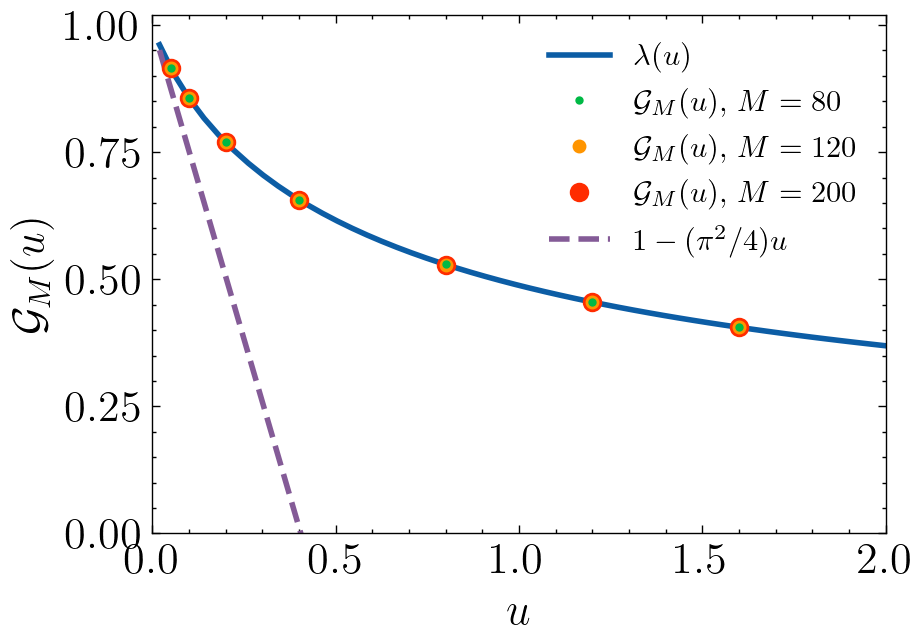
The discussion above isolates the two scaling mechanisms that survive in the continuum limit. The quadratic peak produces the Gaussian window in $\xi$, and the $M$-site support produces the sharp Fourier cutoff $\absolutevalue{p}\leq 1$. An explicit Fourier embedding of the discrete cosine and sine series into the Fourier-window subspace is given in Appendix A.1.1, and the convergence argument is completed in Appendix A.1.3. A numerical illustration of the scaling function $\lambda(u)$ and of the convergence of $\mathcal{G}_{M}(u)$ is given in Fig. 2 in Sec. VII.

Because $\Delta_{M}=M^{2}(2J-V)/J$, the mean drift can be recovered from the defect:

In the optimized setting, define

For $u>0$, the maximizer typically depends on $u$, so derivatives of $\Phi_{M}$ describe how the $u$-optimal family responds when the bias is increased. At $u=0$ the maximization is degenerate since $\mathcal{G}_{M}(0)=1$ for every $\psi$, and the right derivative at zero bias has a direct variational meaning as the optimal mean defect. In particular, we do not interpret $\Phi_{M}^{\prime\prime}(0^{+})$ as an optimization of the variance because the maximizing state typically depends on $u$.

At fixed finite $M$, this endpoint derivative can be obtained directly without differentiating through the degenerate set of maximizers. Let $D^{(M)}$ be the finite-dimensional defect matrix

Since $A_{u}^{(M)}=I_{M}-uD^{(M)}+O_{M}(u^{2})$ in operator norm as $u\downarrow 0$, Rayleigh-Ritz gives

Define the optimal mean defect

The operator-norm expansion leading to Eq. (52) is given in Appendix A.2. By definition (21), we have the exact relation

To extract the large-$M$ asymptotics, it is not necessary to interchange the limit $M\to\infty$ with the right derivative at $u=0$. It is enough to combine the fixed-$u$ scaling limit (48) with a lower bound on $d_{M}$ that holds for every $u>0$. For any fixed $\psi$ and any $u>0$, Jensen’s inequality gives

Let $\psi\in\arg\min_{\phi\in\mathcal{S}_{M}}\mathbb{E}_{\phi}[\Delta_{M}]$. Applying Jensen’s inequality to this choice and using $\mathbb{E}_{\psi}[e^{-u\Delta_{M}}]\leq\mathcal{G}_{M}(u)=e^{\Phi_{M}(u)}$ gives

For each fixed $u>0$, the scaling limit (48) implies $\Phi_{M}(u)\to\Phi(u)=\log\lambda(u)$, hence

See Appendix A.3 for a direct proof. Since $\lambda(0)=1$, we have $\Phi(0)=0$. We define

Appendix A.5 proves directly, without max-differentiation at the degenerate endpoint, that

Therefore, inequality (57) yields

Conversely, fix a real even profile $g\in\mathcal{H}_{\rm W}$ with $\norm{g}_{2}=1$, finite second moment, and a smooth Fourier amplitude compactly supported in $(-1,1)$. Using the explicit embedding in Appendix A.4, we can construct a sequence of states $\psi^{(M)}\in\mathcal{S}_{M}$ whose embedded near-peak profiles approximate $g$ and such that the corresponding mean defects satisfy

Since $d_{M}$ is the minimum of $\mathbb{E}_{\psi}[\Delta_{M}]$ over $\mathcal{S}_{M}$, this gives

Such smooth even Fourier profiles are dense in the even part of $H_{0}^{1}((-1,1))$, which contains the Dirichlet ground-state minimizer in Eq. (67). Optimizing over all such $g$ yields

Combining (60) and (63) shows that $d_{M}=C_{1}+o(1)$ as $M\to\infty$. Substituting this into the exact relation (54) yields

Using $C_{1}=\pi^{2}/4$ from Eq. (59) gives

Thus the main asymptotic result follows. The remaining part of this section gives the Fourier-side interpretation of the coefficient appearing in Eq. (65).

The argument in the previous subsection fixes the coefficient through endpoint bounds. Its value has a simple variational origin in the continuum Fourier-window problem. In Fourier space, multiplication by $\xi$ corresponds to $\mathrm{i}\partial_{p}$. If $g$ is generated by a Fourier-side function $\phi(p)=(2\pi)^{-1/2}\widehat{g}(p)$ supported in $[-1,1]$, then

provided $\phi$ has a square-integrable weak derivative and vanishes at $p=\pm 1$ in the trace sense. This regularity is the Fourier-side expression of a finite second moment. If the Fourier profile does not vanish at the cutoff points $p=\pm 1$, the sharp Fourier cutoff produces a slow real-space tail and the second moment diverges [35, 36, 33, 34]. In this representation, the finite second moment selects profiles whose Fourier amplitude is sufficiently smooth and vanishes at the cutoff points, which is the Dirichlet condition for the associated variational problem. The dimensionless coefficient is therefore the Rayleigh quotient of the Dirichlet Laplacian on $[-1,1]$:

References

- [1] E. Farhi and S. Gutmann, Quantum computation and decision trees, Phys. Rev. A 58, 915 (1998).
- [2] J. Kempe, Quantum random walks: An introductory overview, Contemp. Phys. 44, 307 (2003).
- [3] O. Mulken and A. Blumen, Continuous-time quantum walks: Models for coherent transport on complex networks, Phys. Rep. 502, 37 (2011).
- [4] S. E. Venegas-Andraca, Quantum walks: a comprehensive review, Quantum Inf. Process. 11, 1015 (2012).
- [5] S. Apers, S. Chakraborty, L. Novo, and J. Roland, Quadratic speedup for spatial search by continuous-time quantum walk, Phys. Rev. Lett. 129, 160502 (2022).
- [6] M. Gong, S. Wang, C. Zha, M.-C. Chen, H.-L. Huang, Y. Wu, Q. Zhu, Y. Zhao, S. Li, S. Guo, H. Qian, Y. Ye, F. Chen, C. Ying, J. Yu, D. Fan, D. Wu, H. Su, H. Deng, H. Rong, K. Zhang, S. Cao, J. Lin, Y. Xu, L. Sun, C. Guo, N. Li, F. Liang, V. M. Bastidas, K. Nemoto, W. J. Munro, Y.-H. Huo, C.-Y. Lu, C.-Z. Peng, X. Zhu, and J.-W. Pan, Quantum walks on a programmable two-dimensional 62-qubit superconducting processor, Science 372, 948 (2021).
- [7] A. W. Young, W. J. Eckner, N. Schine, A. M. Childs, and A. M. Kaufman, Tweezer-programmable 2d quantum walks in a hubbard-regime lattice, Science 377, 885 (2022).
- [8] X. Qiang, Y. Wang, S. Xue, R. Ge, L. Chen, Y. Liu, A. Huang, X. Fu, P. Xu, T. Yi, F. Xu, M. Deng, J. B. Wang, J. D. A. Meinecke, J. C. F. Matthews, X. Cai, X. Yang, and J. Wu, Implementing graph-theoretic quantum algorithms on a silicon photonic quantum walk processor, Sci. Adv. 7, eabb8375 (2021).
- [9] N. Konno, Limit theorem for continuous-time quantum walk on the line, Phys. Rev. E 72, 026113 (2005).
- [10] A. D. Gottlieb, Convergence of continuous-time quantum walks on the line, Phys. Rev. E 72, 047102 (2005).
- [11] C. Cedzich, A. Joye, A. H. Werner, and R. F. Werner, Exponential tail estimates for quantum lattice dynamics, Ann. Henri Poincaré (2025).
- [12] T. Machida, Phase transition of a continuous-time quantum walk on the half line, Quantum Inf. Process. 23, 243 (2024).
- [13] E. H. Lieb and D. W. Robinson, The finite group velocity of quantum spin systems, Commun. Math. Phys. 28, 251 (1972).
- [14] M. C. Tran, A. Y. Guo, C. L. Baldwin, A. Ehrenberg, A. V. Gorshkov, and A. Lucas, Lieb-robinson light cone for power-law interactions, Phys. Rev. Lett. 127, 160401 (2021).
- [15] Z. Wang and K. R. Hazzard, Tightening the lieb-robinson bound in locally interacting systems, PRX Quantum 1, 010303 (2020).
- [16] C.-F. (Anthony) Chen, A. Lucas, and C. Yin, Speed limits and locality in many-body quantum dynamics, Rep. Prog. Phys. 86, 116001 (2023).
- [17] H. Touchette, The large deviation approach to statistical mechanics, Phys. Rep. 478, 1 (2009).
- [18] R. Chetrite and H. Touchette, Nonequilibrium Markov processes conditioned on large deviations, Ann. Henri Poincaré 16, 2005 (2015).
- [19] P. M. Preiss, R. Ma, M. E. Tai, A. Lukin, M. Rispoli, P. Zupancic, Y. Lahini, R. Islam, and M. Greiner, Strongly correlated quantum walks in optical lattices, Science 347, 1229 (2015).
- [20] C. Gross and W. S. Bakr, Quantum gas microscopy for single atom and spin detection, Nat. Phys. 17, 1316 (2021).
- [21] A. Di Carli, C. Parsonage, A. La Rooij, L. Koehn, C. Ulm, C. W. Duncan, A. J. Daley, E. Haller, and S. Kuhr, Commensurate and incommensurate 1D interacting quantum systems, Nat. Commun. 15, 474 (2024).
- [22] S. Richard, A. Suzuki, and R. T. de Aldecoa, Quantum walks with an anisotropic coin II: scattering theory, Lett. Math. Phys. 109, 61 (2019).
- [23] A. Mandal, R. S. Sarkar, S. Chakraborty, and B. Adhikari, Limit theorems and localization of three-state quantum walks on a line defined by generalized grover coins, Phys. Rev. A 106, 042405 (2022).
- [24] T. Tate, An eigenfunction expansion formula for one-dimensional two-state quantum walks, Ann. Funct. Anal. 13, 65 (2022).
- [25] M. MAEDA, H. SASAKI, E. SEGAWA, A. SUZUKI, and K. SUZUKI, Dispersive estimates for quantum walks on 1D lattice, J. Math. Soc. Jpn. 74, 217 (2022).
- [26] H. Abdul-Rahman and G. Stolz, Exponentially decaying velocity bounds of quantum walks in periodic fields, Commun. Math. Phys. 403, 1297 (2023).
- [27] J. G. Van der Corput, Zur Methode der stationaren Phase. Erste Mitteilung Einfache Integrale, Compos. Math. 1, 15 (1935).
- [28] A. Erdélyi, Asymptotic representations of fourier integrals and the method of stationary phase, J. Soc. Ind. Appl. Math. 3, 17 (1955).
- [29] K. Liu, M. Nakagawa, and M. Ueda, Maxwell’s demon for quantum transport, Phys. Rev. A 113, 022436 (2026).
- [30] H. Widom, Asymptotic behavior of block toeplitz matrices and determinants. ii, Adv. Math. 21, 1 (1976).
- [31] T. Claeys, G. Glesner, A. Minakov, and M. Yang, Asymptotics for averages over classical orthogonal ensembles, Internat. Math. Res. Notices. 2022, 7922 (2021).
- [32] G. Strang and S. MacNamara, Functions of difference matrices are toeplitz plus hankel, SIAM Rev. 56, 525 (2014).
- [33] D. Slepian and H. O. Pollak, Prolate spheroidal wave functions, fourier analysis and uncertainty — i, Bell Syst. Tech. J. 40, 43 (1961).
- [34] H. J. Landau and H. O. Pollak, Prolate spheroidal wave functions, fourier analysis and uncertainty — ii, Bell Syst. Tech. J. 40, 65 (1961).
- [35] H. J. Landau and H. Widom, Eigenvalue distribution of time and frequency limiting, J. Math. Anal. Appl. 77, 469 (1980).
- [36] H. Widom, Asymptotic behavior of the eigenvalues of certain integral equations. II, Arch. Ration. Mech. Anal. 17, 215 (1964).
- [37] M. G. Krein and M. A. Rutman, Linear operators leaving invariant a cone in a Banach space, Uspekhi Mat. Nauk 3, 3 (1948).
- [38] W. Ritz, Uber eine neue methode zur losung gewisser variationsprobleme der mathematischen physik, J. Reine Angew. Math. 1909, 1 (1909).
- [39] J. K. L. MacDonald, Successive approximations by the rayleigh-ritz variation method, Phys. Rev. 43, 830 (1933).
- [40] H. Kim, W. Lee, H.-G. Lee, H. Jo, Y. Song, and J. Ahn, In situ single-atom array synthesis using dynamic holographic optical tweezers, Nat. Commun. 7, 13317 (2016).
- [41] S. Bose, Quantum communication through an unmodulated spin chain, Phys. Rev. Lett. 91, 207901 (2003).
- [42] M. Christandl, N. Datta, A. Ekert, and A. J. Landahl, Perfect state transfer in quantum spin networks, Phys. Rev. Lett. 92, 187902 (2004).
- [43] A. Kay, Perfect, efficient, state transfer and its application as a constructive tool, Int. J. Quantum Inf. 08, 641 (2010).
- [44] B. Nachtergaele and R. Sims, Lieb-Robinson bounds and the exponential clustering theorem, Commun. Math. Phys. 265, 119 (2006).
- [45] M. B. Hastings and T. Koma, Spectral gap and exponential decay of correlations, Commun. Math. Phys. 265, 781 (2006).
- [46] F. Campaioli, S. Gherardini, J. Q. Quach, M. Polini, and G. M. Andolina, Colloquium: Quantum batteries, Rev. Mod. Phys. 96, 031001 (2024).
- [47] J. Yu, S. Wang, K. Liu, C. Zha, Y. Wu, F. Chen, Y. Ye, S. Li, Q. Zhu, S. Guo, H. Qian, H.-L. Huang, Y. Zhao, C. Ying, D. Fan, D. Wu, H. Su, H. Deng, H. Rong, K. Zhang, S. Cao, J. Lin, Y. Xu, C. Guo, N. Li, F. Liang, G. Wu, Y.-H. Huo, C.-Y. Lu, C.-Z. Peng, K. Nemoto, W. J. Munro, X. Zhu, J.-W. Pan, and M. Gong, Experimental demonstration of a maxwell’s demon quantum battery in a superconducting noisy intermediate-scale quantum processor, Phys. Rev. A 109, 062614 (2024).
- [48] P. Campagne-Ibarcq, E. Flurin, N. Roch, D. Darson, P. Morfin, M. Mirrahimi, M. H. Devoret, F. Mallet, and B. Huard, Persistent control of a superconducting qubit by stroboscopic measurement feedback, Phys. Rev. X 3, 021008 (2013).
- [49] A. C. Doherty, S. Habib, K. Jacobs, H. Mabuchi, and S. M. Tan, Quantum feedback control and classical control theory, Phys. Rev. A 62, 012105 (2000).
- [50] M. Nakagawa and M. Ueda, Topology of discrete quantum feedback control, Phys. Rev. X 15, 021016 (2025).
- [51] E. J. Nyström, Über die praktische auflösung von integralgleichungen mit anwendungen auf randwertaufgaben, Acta Math. 54, 185 (1930).
- [52] R. Jentzsch, Über integralgleichungen mit positivem kern., J. Reine Angew. Math. 1912, 235 (1912).
- [53] H. Hanche-Olsen and H. Holden, The kolmogorov–riesz compactness theorem, Expo. Math. 28, 385 (2010).