

Measured Joules, Learned Routes: Learning to Route for Energy-Efficient LLM Serving
Abstract.
Large language models (LLMs) and agentic AI systems are creating rapidly growing inference energy demands as model sizes grow and reasoning trajectories extend. While in practice, many queries do not require the capabilities of the largest available model, and routinely directing such queries to a high-capability model can introduce unnecessary, considerable computation and energy consumption. In this paper, we investigate whether adaptive routing across a heterogeneous pool of LLMs can reduce this energy burden without substantially compromising task performance. We design a language-model-based router that reads in each query and selects an answer model from a fixed candidate pool. The candidate models are first profiled through an offline tournament that records their correctness, latency, power, and GPU energy for each query. Using these measurements, the router is trained through supervised fine-tuning followed by group relative policy optimization (GRPO) with the tailored paradigms. Results demonstrate that learned routing can selectively allocate expensive model capacity based on query contexts, and effectively improve the accuracy–energy trade-off of multi-LLM serving. Across seven benchmark tasks, we also observe a sharp accuracy–energy phase transition among routers, providing practical insights in terms of striking the energy efficiency while still keeping LLM performance.
1. Introduction
Artificial intelligence (AI), particularly large language models (LLMs), already places substantial demands on computing infrastructure and its electricity supply. Inference is becoming the central part of this energy burden. As deployed models with billions or trillions of parameters repeatedly process requests throughout their operational lifetime, so even modest energy costs per response accumulate at service scale (Oviedo et al., 2026; Chung et al., 2026a). Longer reasoning outputs and agentic workflows can increase this demand further by generating more tokens and invoking models multiple times for a single user request (Chung et al., 2026b). These workloads make inference efficiency an important concern for sustainable AI serving with regard to cutting down energy spent answering queries while preserving task performance.
As current LLMs vary by model sizes, specialized areas, and associated computing demands, model routing offers one approach to this challenge. Instead of assigning every query to the same LLM, in practice, a router can select an answer model from a heterogeneous pool according to the query’s requirements and characteristics (Song et al., 2025; Li et al., 2026). As modern AI models differ to a significant extent in their capabilities across reasoning, coding, and knowledge-intensive tasks, it creates opportunities to allocate computational effort selectively (Hu et al., 2024). Always sticking to a high-capability model can spend unnecessary energy on queries that a smaller model could answer correctly, whereas always using a small model can sacrifice accuracy on more demanding inputs. Query-dependent LLM model selection therefore offers a way to exploit model diversity and adjust the quality-cost trade-off (Ong et al., 2025; Jitkrittum et al., 2026; Hu et al., 2024).
However, making routing effective and tailored for energy reduction presents a few challenges. Indeed, the cost of a model invocation depends on both models and queries. Input and output lengths, hardware, and serving configurations affect energy consumption, so current practices like parameter counts, API prices, and fixed model-level costs do not fully expose the joules consumed by the underlying generation task (Wilkins et al., 2024; Chung et al., 2026a). This issue becomes especially important in agentic LLM systems, where one user request may trigger multiple model calls for planning, tool use, verification, and revision (Yang et al., 2026). Moreover, an energy-centric router shall be able to judge and evaluate whether a candidate will answer correctly before observing its output. Reducing energy by systematically choosing weaker models can undermine the service’s purpose, and the useful routing requires learning when additional model capacity is warranted. Another concern is routing itself consumes computation, while most of recent works on router design may not distinguish the selected model’s consumption from the overhead of making and executing that decision (Ong et al., 2025; Jitkrittum et al., 2026).
In this work, we study whether a tailored small language model can learn the unique energy-aware routing policy from measured AI serving outcomes. To achieve this router training, we first conduct an offline tournament in which every candidate answer model processes every training question, producing logs of correctness, latency, power, and GPU energy. These logs define an oracle route and a gated reward, where we propose that incorrect answers receive a fixed penalty, while correct answers receive a reward reduced by the selected model’s within-query energy rank. Built upon recent advancements in agentic post-training paradigms (Luo et al., 2025; Jiang et al., 2025) together with this novel profiling data, the routing controller is trained through supervised fine-tuning (SFT) followed by group relative policy optimization (GRPO) (Shao et al., 2024), including a variant regularized toward the SFT policy. Rather than guided to output complete final answers, based on query contexts, we design the training paradigm to let the router only output the routing decision, which is both lightweight and highly generalizable after finetuning on the small energy-aware datasets. During training and evaluation, model outcomes are replayed from the tournament logs, so answer models do not need to be invoked repeatedly. Figure 1 illustrates our proposed router training and implementation workflow.

This work makes three main contributions. First, we formulate LLM model routing around measured GPU energy rather than model size or monetary price alone. Second, we illustrate a practical way of profiling LLM energy and performance during inference, and develop a compact LLM-based routing controller trained through an SFT-to-RL pipeline under a gated accuracy-energy reward. Third, we evaluate proposed and classical model routers on a nine-model pool across a diverse held-out mixture of seven benchmarks. Results indicate a sharp accuracy-energy transition near 60% accuracy, where LLM models below this region can remain relatively inexpensive, whereas higher accuracy requires substantially more frequent use of capable models. Our proposed policy trained via the mixed KL-GRPO scheme reaches similar accuracy as UniRoute (Jitkrittum et al., 2026) , while consistently using about less mean answer energy ( vs. ). Ablation studies also indicate interesting observations regarding reward selection, model collapse, and tradeoff between AI performance and energy footprints. We will open-source the proposed router after reviewing period.
1.1. Related Work
1.1.1. Energy-efficient LLM inference
Due to the surging energy demand associated with AI usage, research start to investigate the power and energy impact of AI training and AI serving (Chung et al., 2026a; Li et al., 2024). Inference energy costs are alarming as agentic tasks involve complicated reasoning loops, long reasoning chains, and tendency of using larger sizes of LLMs (Luccioni et al., 2024). Researchers have identified hardware selection (Wilkins et al., 2024), AI model training (You et al., 2023), LLM model caching and serving strategies (Wang et al., 2025; He et al., 2025), preemptive power management (Patel et al., 2024) as opportunities of energy reduction. Prior work has measured substantial variation in LLM inference energy across tasks, models, and deployment configurations (Chung et al., 2026a; Oviedo et al., 2026). Such measurement literature shows that energy depends on model size, batching, hardware, precision, and generation length. For instance, most routers shown in Table 2 still optimize accuracy, embedding similarity, or API-style cost proxies rather than measured GPU energy on the serving stack. GreenServ (Ziller et al., 2026) is the main exception among our baselines because it explicitly trades accuracy against normalized inference cost in the bandit reward. We evaluate classical and learned routers on the same held-out mix with logged GPU energy, power, and latency, and we study how reward shaping and RL reshape the accuracy–energy frontier over a multi-model local pool.
1.1.2. Routers for AI Serving
A growing line of work considers practical serving systems, and treats model selection as a first-class inference problem instead of fixing one backend for every query. Most of these routers are designed to optimize efficiency (Jitkrittum et al., 2026), while outputs with least token outputs may not be directly translated to energy consumption. RouterBench formalizes this setting with a large offline benchmark of per-model outcomes and popular routing baselines (Hu et al., 2024). Among them, -nearest-neighbour routing scores each candidate from the error rates of models on embedding neighbours of the test prompt. UniRoute (Jitkrittum et al., 2026) represents each LLM through its errors on representative prompt clusters, so a model can be scored and routed to even when it was not in the original training pool. Smoothie (Guha et al., 2024) takes a label-free route. It embeds each candidate’s prompt–output pair and estimates per-sample quality without correctness labels on the routing split. RouteLLM (Ong et al., 2025) learns a binary strong–weak router from preference data and thresholds a win probability to trade cost against quality. In our design, we adapt that rule to a strong–weak pair from the local candidate pool rather than the paper’s API checkpoints. GreenServ (Ziller et al., 2026) targets energy-aware serving. It models routing as a contextual bandit and uses LinUCB (Li et al., 2010) is a classical bandit-based approach that maintains a disjoint linear reward model per arm and explores with an uncertainty bonus. GreenServ’s reward mixes accuracy with normalized inference cost, which is close in spirit to our gated accuracy–energy objective, while our controller is a learned language model rather than a hand-built feature vector.
The broader AI serving system’s goal is not a single router knob, posing challenges to router design. Indeed, agentic serving has two coupled controls. One is which model answers a query. The other is how much reasoning that call is allowed to spend. Most routers named above decide only the first. ARES (Yang et al., 2026) decides the second, and it does so adaptively. It chooses how much reasoning effort an agent should spend on the current query, so harder items can think longer and easier items can stop sooner. It does not assign one fixed thinking budget to every call. That split is part of what motivates this work. A fixed model wastes energy on easy items and still fails hard ones and a fixed thinking budget has the same problem inside one model. ARES is the closest prior statement of that second failure, and it treats reasoning effort as something the system should choose rather than freeze. Our controller attacks the first control with a small language model and a gated accuracy–energy reward on measured GPU logs. Together the two controls point to the same end goal. Agentic inference should spend compute only when the task justifies it.
1.1.3. Agentic RL
Training the router as a policy rather than only as a classifier connects our setup to agentic RL for language models. Recent advances have shown effectiveness of RL in post training which go beyond text imitation usually happening in SFT approaches. AgentLightning (Luo et al., 2025) is an agent training framework that wraps rollout generation and policy optimization for multi-step workflows. Hugging Face TRL (von Werra et al., 2020) is a separate library that implements GRPO and related on-policy algorithms for language models. We explored both stacks on the same offline tournament reward. Our reported SFT, GRPO, and KL-GRPO numbers use TRL, so training, checkpoints, and held-out evaluation stay in one consistent pipeline. Agent Lightning experiments served as a cross-check on the same reward design rather than as a second training path in the main tables. The distinction between supervised fine-tuning (SFT) and on-policy RL matters here (Yu et al., 2026). Prior analyses show that RL can improve exploration and reward shaping beyond imitation of static routing labels, while SFT remains a stable warm start (Chu et al., 2025). To that end, in this work we study whether RL on replayed tournament rewards can learn when extra answer-model cost is worth higher accuracy under measured energy constraints.
2. Problem Formulation
2.1. Heterogeneous model pool
For modern AI model serving, it is hard to apply one LLM model fit all inputs. This is due to the fact that it becomes challenging to strike a balance between being accurate on hard items and staying efficient on easy queries. For instance, a small, open-weight model generates few tokens and spends little energy, but it can fail queries which need more model and reasoning capacity. Whereas a large, reasoning-based model does the reverse, because they may overthink, and can waste significant amount of joules on items a smaller model would have easily answered (Zhao et al., 2026).
To this end, we study a serving system that selects one answer LLM for each incoming query. Let denote a fixed pool of candidate LLMs, and let index the available routes. A query context contains the question and any metadata provided to the router. The routing policy selects a candidate index , after which model generates an answer . The router makes the model-selection decision; the selected candidate performs the task. Each evaluated query involves one routing decision and one answer-model outcome. Multi-turn recovery and tool use could also be applied to our framework with proper extensions.
The pool of candidate LLMs is heterogeneous by design, and the model card is illustrated in Table 1. Candidates differ in model family, parameter count, and reasoning style, from sub-billion Qwen2.5 drafts through mid-size models such as Gemma2-2B, Qwen2.5-7B, and Llama 3.1 8B, up to DeepSeek-R1 8B and 32B. That spread is what makes routing meaningful. These differences create opportunities for query-dependent selection, since a model that is effective for one task need not offer the best accuracy–energy trade-off for another. For example, Figure 2 shows a GSM8K query answered correctly by Qwen2.5-0.5B using and by DeepSeek-R1-8B using , while Llama 3.1-8B answers incorrectly using . For this question, though Llama model has larger size, its overthinking and extra steps around equation modeling causes both inefficient and inaccurate inference. Such an example motivates measuring outcomes for each query-energy-model triplet rather than inferring suitability from model size alone. We assume all answer models are open-weight checkpoints served locally through Ollama on that device, so each candidate can be invoked under the same power logger rather than billed as a separate API price.
GSM8K, question 31. Gunter is trying to count the jelly beans in a jar. He asks his friends how many they think are in the jar. One says 80. Another says 20 more than half the first one. A third says 25% more than the first one. What is their average guess?
Qwen2.5-0.5B (correct) J | s Answer: 80 Response: “First, let’s calculate each friend’s guess: (1) The first friend guesses 80 jelly beans. (2) The second friend guesses 20 more than half of 80, which is . (3) The third friend guesses 25% more than the first one, which is . The average is .”
Llama 3.1-8B (wrong) J | s Answer: 106.67 Response: “Let’s denote Gunter’s friend who said 80 as F1, the second friend as F2, and the third friend as F3. F2 F1. F3 F1. Now we can find the average of their guesses by adding up all three guesses and dividing by 3: Average = (F1 + ((1/2) * F1 + 20) + (1.25 * F1))/3 Combine like terms. Average = (F1 + (0.5 * F1) + 20 + (1.25 * F1))/3 Simplify the numerator. Average = (3.75 * F1 + 20)/3 Now we can plug in the value of F1, which is 80. Average = (3.75 * 80 + 20)/3 Multiply 3.75 and 80. Average = (300 + 20)/3 Add 300 and 20. Average = 320/3 Divide 320 by 3. Average = 106.67”
DeepSeek-R1-8B (correct) J | s Answer: 80 Response: “The first friend guesses 80 jelly beans. The second friend guesses 20 more than half of the first guess: half of 80 is 40, so . The third friend guesses 25% more than the first guess: 25% of 80 is 20, so . The average is .”
2.2. Recorded outcomes and energy measurement
For query and candidate , let be the recorded answer and its reference. We denote correctness by
| (1) |
where is the evaluator for benchmark . This notation covers task-specific answer matching and code-test evaluation without requiring exact and literal string equality. Let , , and denote the each answer call ’s incremental GPU energy in joules, wall-clock duration in seconds, and mean incremental GPU power in watts, respectively.
The candidate models are served locally through Ollama on NVIDIA A100-SXM4-80GB GPUs with tensor parallelism. During profiling, the logger polls board power through NVML using pynvml at a interval and subtracts an idle-power baseline. We adopt nvidia-ml-py bindings, which read the same device counters as nvidia-smi. Let denote the board power trace and the baseline associated with the query call , the measurement quantities of power, energy, and duration are modeled as
| (2) | ||||
| (3) | ||||
| (4) |
The energy integral is estimated from the sampled trace. Note these quantities describe idle-subtracted GPU consumption within the measured query call interval, which is the core energy associated with AI inference. They do not represent total server or data-center-level energy consumption.
We first profile AI model’s energy and performance through an offline tournament of mild size, which records the outcomes of the candidate models on the collected questions. With given query input , the per-query record is profiled as
| (5) |
These are realized outcomes of the underlying LLM inference generations. Replaying a record reproduces that recorded outcome, rather than estimating the answer model’s stochastic behavior or measurement variation. The complete outcome vector provides feedback for all candidates on a training query, although the learned policy selects only one candidate at inference time.
2.3. Energy-Aware AI serving objectives
In this work, we explore the possibilities of meeting LLM service objectives at low energy cost. On a fixed logged dataset of queries, the expected accuracy and answer energy of a feasible routing policy are
| (6a) | ||||
| (6b) | ||||
For deterministic routing, these expressions reduce to averages of the selected candidates’ outcomes. For sampled decisions, the corresponding sample averages estimate these expectations. Handling of invalid controller outputs is discussed in Section 3.1.
One design to handle the desired accuracy-energy trade-off is
| (7) |
where is an average answer-energy budget in joules per query. This constraint expresses a service goal, not a guarantee made by the training algorithm. The reported method instead optimizes the gated rank-based surrogate defined in Section 3.2 and evaluates its resulting accuracy and measured answer energy. Problem (7) can be treated as a single-step contextual decision problem. A contextual-bandit formulation accommodates either a classical or a text-conditioned neural policy. In addition, our logged training data provide detailed outcomes for every candidate. We therefore distinguish the routing problem, the controller’s representation, and the feedback used to train it.
We note with the addition of the router policy , the complete serving energy also depends on the controller and deployment costs, including model loading and residency under the chosen serving configuration. Those costs is measured use the consistent metric to establish end-to-end savings, and they are not supplied by the lookup of alone. More importantly, as LLM’s consumed energy are strongly dependent on input queries and output contexts, it requires dedicated design and investigation of the router.
| Model | Nominal Size | ARC Acc. | Energy (J) |
|---|---|---|---|
| Qwen 2.5 | 0.5B | 0.314 | 66.1 |
| Qwen 2.5 | 1.5B | 0.665 | 84.3 |
| Qwen 2.5 | 3B | 0.727 | 131.7 |
| Phi-3 Mini | 3.8B | 0.803 | 170.5 |
| Gemma 2 | 2B | 0.722 | 56.2 |
| Qwen 2.5 | 7B | 0.871 | 140.8 |
| Llama 3.1 | 8B | 0.803 | 196.1 |
| DeepSeek-R1 | 8B | 0.932 | 2142.2 |
| DeepSeek-R1 | 32B | 0.939 | 3307.9 |
| Policy | Accuracy | Reward | Duration (ms) | Model Energy (J) | Power (W) |
| always_smallest | 0.189 | - | 3780 | 91.8 | 23.2 |
| always_medium | 0.791 | - | 28672 | 4127.9 | 125.9 |
| always_large | 0.735 | - | 25706 | 5112.4 | 174.5 |
| K-NN | 0.790 | - | 23366 | 3697.6 | 121.3 |
| UniRoute | 0.618 | - | 15371 | 2192.2 | 84.8 |
| Smoothie | 0.599 | - | 9269 | 1070.6 | 59.4 |
| RouteLLM | 0.721 | - | 25053 | 4958.6 | 170.3 |
| GreenServ () | 0.567 | - | 5584 | 277.0 | 41.4 |
| SFT () | 0.502 | 0.400 | 7821 | 822.8 | 45.9 |
| KL-GRPO (sft , rl , step 500) | 0.591 | 0.686 | 10932 | 1339.8 | 47.1 |
| KL-GRPO (sft , rl , step 1500) | 0.609 | 0.720 | 13118 | 1691.9 | 55.2 |
| GRPO (sft , rl , step 750) | 0.584 | 0.666 | 7942 | 811.8 | 48.5 |
| GRPO (both , step 1000) | 0.573 | 0.612 | 6002 | 297.0 | 46.8 |
3. Agentic Learning to Route
3.1. Router’s environment
To fully release the routing controller’s effectiveness, we propose to utilize a lightweight, finetuned LLM in a text-conditioned approach. Its role is to interpret a query and select a candidate from the fixed pool, using a smaller LLM than most of the candidate answer models. The controller prompt contains the question like in Figure 9, a fixed legend mapping labels to candidate indices, and an optional difficulty field when available. Recorded correctness and energy are regarded as training feedback rather than inputs supplied to the controller when selecting a model.
Let denote the probability of a controller completion given query context , and let parse its route label into an index in . The induced route probabilities are
| (8) |
This separates probabilities over generated texts from probabilities over candidate models. The reported variants use either a short rationale with a Choice: <letter> field or a choice-only completion. Both formats produce the same model-selection action. An un-parseable output is an invalid action and receives a negative training reward. If multi-turn routing is enabled, the router also sees any prior user-assistant turns on the same item, the current turn number, the model chosen last time, and whether that attempt was correct. The router can output Stop when a satisfactory answer already exists and does not require to route to candidate LLMs. In all reported experiments we use a single routing turn per question, so each item produces one letter choice. Probability on invalid outputs is separate from the valid-route probabilities in Eq. (8).
The tournament contains approximately collected questions from MMLU, GSM8K, BBH, ARC Challenge, HellaSwag, MATH-500, and HumanEval. The reported training and held-out subsets contain and questions, respectively; benchmark counts are given in Table 5 in Appendix. The training subset supplies oracle labels and policy rewards. We use Qwen2.5-1.5B-Instruct as a text-conditioned routing controller, and find it achieve desired post-training behaviors with respect to routing decisions. During policy optimization, the controller generates new completions, but answer-model outcomes are retrieved from the fixed training records. Thus, router sampling is on-policy with respect to the rollout controller, while its environmental feedback is replayed.
3.2. Router reward design
To ensure in the RL post-training, the router can effectively evaluate the input queries’ contexts and make decisions, we come up with a ranking-based reward for energy, which is in the same scale as of performance reward. Such a reward combines task correctness with preferences over inference costs (e.g., energy, task completion time and etc). For query and candidate , denotes correctness, denotes answer latency in seconds, and denotes mean incremental GPU power in watts. The measured answer energy is expressed in joules.
We derive a bounded energy penalty from the ascending rank of among the candidates for the same query:
| (9) |
With distinct energies, zero corresponds to the cheapest candidate and one to the most expensive. For example, energies of , , , and produce penalties of , , , and . denotes rank throughout. It is distinct from energy . Ranking bounds the training penalty but discards the magnitude of differences in joules.
Let denote nonnegative cost coefficients associated with session duration, energy rank, and average GPU power. The general gated reward is
| (10) |
Latency, energy, and power describe related but different aspects of a session call. The same energy can be consumed over different durations and at different mean power levels. Thus, separate latency and power coefficients can express preferences over those quantities, but an average-power penalty alone does not enforce an instantaneous device or rack power limit. We distinguish this general reward form from the configuration used in the reported experiments as follows.
Reported experimental configuration.
In our paper, all reported reward configurations set to focus on energy analysis, with and . The active training reward therefore reduces to
| (11) |
Latency and mean GPU power are consequently measured and reported but do not contribute to the optimization signal in these runs. The oracle and policy-optimization descriptions below use this specialization. Invalid controller outputs and unavailable outcomes receive a separate negative penalty rather than the valid-route score above. Equivalently, the active reward can be expressed as
| (12) |
Our reward design distinguishes the costs of correct routes, while it assigns equal reward to cheap and expensive failures. It is an empirical learning surrogate instead of a guarantee of meeting the joule budget in Eq. (7). Evaluation counts measured answer energy for successful and unsuccessful answers alike. Joint optimization with nonzero latency or power weights is not demonstrated by the reported experiments.
3.3. Oracle construction and supervised initialization
For each training query, the oracle target is selected from
| (13) |
where is the coefficient used during target construction. Under the reported positive coefficients , every correct route receives a larger reward than every incorrect route. The oracle therefore selects a lowest-energy correct candidate whenever one exists. Changing the positive coefficient within this range does not change that hard target if the logs and tie-breaking rule are fixed. For , correct candidates tie, and the draft’s accuracy-only configuration selects the largest correct model. When all candidates are wrong, every valid route ties under the reward.
Let be the target completion encoding the selected route in the chosen output format. Supervised fine-tuning initializes the controller by minimizing the completion negative log likelihood
| (14) |
where indexes the training queries. We can include two variations of the target during SFT. In the choice-only variant, the target contains the route field; in the rationale variant, it also contains an explanation. The resulting checkpoint is evaluated as an SFT baseline and initializes policy optimization. SFT learns to imitate target completions, whereas the next stage uses the rewards of the controller’s sampled decisions.
3.4. Group-relative policy optimization
We fine-tune the controller using GRPO (Shao et al., 2024), which is based on groupwise comparisons instead of using a separate critic model. For each training query , a rollout policy samples completions . Each completion is parsed and scored using its selected candidate’s logged outcome and coefficient , or the invalid-action penalty. Denote these completion rewards by . Their group statistics and advantages are
| (15) | ||||
| (16) |
where stabilizes the denominator. A completion receives positive advantage when its reward exceeds the group mean. If all group rewards are equal, all advantages are zero and that group supplies no reward-driven update.
At the completion level, the clipped policy surrogate is expressed using importance sampling ratio
| (17) |
with the resulting loss function
| (18) |
where controls ratio clipping and is distinct from the advantage stabilizer . This surrogate favors higher-reward completions while limiting the incentive for large policy-ratio changes.
The KL-regularized variant additionally anchors the controller to the SFT reference distribution . At the distribution level its regularized objective is
| (19) |
with regularization coefficient . This expression concerns controller completions rather than the marginal distribution over model indices in Eq. (8). Note KL regularization discourages departure from the reference policy. It does not by itself guarantee diverse routing or prevent concentration on a single candidate. Some configurations center rewards by subtracting a query-specific mean candidate reward. If the same scalar is subtracted from every reward before the group normalization in Eq. (16), it cancels from the advantages. Such centering is therefore distinct from any additional reward scaling or clipping used by the trainer.
3.5. Training configurations and evaluation
In this paper, we unify and use TRL to conduct main SFT, GRPO, and KL-GRPO post-training (von Werra et al., 2020). Policy optimization starts from the corresponding SFT checkpoint, and samples multiple controller completions per training prompt. The main reported configuration uses and as we find these hyperparameters give the best overall SFT and RL performances. The experiments also examine matched coefficients and alternative checkpoints. These coefficients identify the oracle-construction and policy-reward settings, respectively. Their effects on hard targets, sampled rewards, and learned policies should be distinguished. The output format is also part of each configuration, where choice-only and rationale-generating controllers have different generation costs, and should be compared with their matching SFT initializations.
On held-out queries, the router can be treated as the lightweight add-on to inference engines, where it selects a LLM model and the evaluator retrieves that candidate’s stored outcome. We report accuracy, mean answer-model energy, latency, power, and model-selection frequencies. Reward comparisons require a common evaluation coefficient: reward values computed with different are different metrics even when the policies share an SFT initialization. Accuracy and measured joules provide the primary comparison across configurations and baselines.
The replay protocol isolates model-selection behavior on a fixed outcome table. It does not measure live changes in answer generation, model-loading cost, queueing, or concurrent serving. Controller measurements and answer-model measurements must therefore be distinguished when discussing complete serving costs. The evaluation addresses single-turn routing on the profiled pool. Adaptation to new deployment conditions and multi-turn agent workflows would require additional experiments.

4. Numerical Studies
4.1. Simulation setup
We evaluate routing policies on a mixed held-out set drawn from seven standard LLM benchmarks that span knowledge, reasoning, math, and code: MMLU (Hendrycks et al., 2020), GSM8K (Cobbe et al., 2021), BBH (Suzgun et al., 2023), ARC Challenge (Clark et al., 2018), HellaSwag (Zellers et al., 2019), MATH-500 (Lightman et al., 2024), and HumanEval (Chen et al., 2021). These tasks stress different answer-model costs, from short multiple-choice items to long generative math and code solutions, which is what makes energy-aware routing nontrivial on the shared nine-model pool.
Power measurements are based on NVML11 1 https://docs.nvidia.com/deploy/nvml-api/. To keep energy and performance comparable across runs, we place all router training and inference on instances of 1x NVIDIA A100-SXM4-,GB GPU. Answer models are served locally with Ollama on that device. The routing controller is trained and run with Hugging Face Transformers and TRL on the same GPU. Offline tournament collection used a separate machine with the same A100-SXM4-,GB specification. During each answer-model generation we poll board power at a interval via pynvml, subtract a short idle baseline, and record instantaneous effective power in watts. Effective energy for the call is as defined in Eq. (3), and latency is the wall-clock duration of the same generation. Table 2 reports mean accuracy together with measured duration, energy, and power summaries.
All methods in Table 2 are scored on the same 913 held-out test questions covering a spectrum of difficulty and categories. Scoring is an offline lookup from pre-logged tournament outcomes, so no live answer models are called at evaluation time.
K-NN estimates per-model error from embedding neighbours on the train split. UniRoute matches the prompt to a train K-means cluster and uses per-cluster error plus a cost term. Smoothie is label-free and scores candidates from embeddings of . Unlike the others, Smoothie uses all logged generations on the test item to decide, so we treat it as an output-informed diagnostic rather than a deployable pre-generation router. We still charge only the chosen model’s energy. GreenServ is a local LinUCB adaptation using task, semantic-cluster, and complexity features. Its reward is and is warmed on train and frozen before test. It is not the paper’s online serving stack. RouteLLM is a binary router over two fixed answer models, not a classifier over the full pool. We set the strong arm to DeepSeek-R1-32B and the weak arm to the smallest pool model, train a prompt classifier for on train outcomes, and route to the strong arm when . Fixed-model baselines always route every question to one predetermined answer model (always-smallest, always-medium, or always-large).
Table 2’s methods and results can be split into three categories. High-accuracy part is K-NN and always-medium, near at about –. Always-large and RouteLLM spend even more and do worse. The mid-accuracy band is UniRoute, Smoothie, and our GRPO runs, about to at to . The cheap accuracy band is GreenServ and matched GRPO , about at about –. SFT sits below that mid accuracy band. Always-smallest is cheap in energy but achieves poor accuracy.
Reward parameters.
We instantiate Eq. (11) with , , , and energy-rank mode for in Eq. (9), so the training signal is the gated rank surrogate rather than raw joules. Baselines do not train on this gated reward, so the Reward column is blank for them. For SFT and TRL the Reward column is therefore when and when . SFT uses . The runs use . Matched GRPO uses at both stages. Therefore, the Reward column should only be compared among SFT and RL inside that block. Acc., duration, energy, and power are the columns to compare across the whole table.
4.2. Results and discussion
Accuracy–energy trade-off among routers
Figure 4 plots mean answer energy against held-out accuracy for the multi-model routers and learned controllers in Table 2. Blue markers are TRL sweeps over (von Werra et al., 2020). Among these methods, policies near accuracy generally report higher mean answer energy than policies that remain below that range by relying more on smaller candidate models. The additional energy is associated with more frequent selection of higher-capacity models when the query requires it. This comparison is restricted to the routers and learned controllers under study, and does not describe every fixed model in the candidate pool. Under that scope, KL-GRPO step 1500 nearly matches UniRoute ( vs. ) at about lower mean answer energy ( vs. ), and GRPO step 750 is close to Smoothie ( vs. ) at about lower mean answer energy ( vs. ).
Role of a mid-size fixed arm
A single mid-size model can look strong in aggregate. For instance, Always-Qwen2.5-7B reaches at on the same held-out pool (Appendix Table 8), yet it falls to on BBH, so locking every query to 7B can be a weak suite-wide policy even when the overall mean is high. Our question is not whether one fixed arm can beat a router on the mean, but whether a controller can allocate capacity across the pool. Figure 3 shows that the learned and classical routers still call 7B when it helps. About one third of GreenServ traffic, about for GRPO step 750, and about for both KL-GRPO step 1500 and UniRoute use that arm. In that sense 7B is a useful pool member, not a substitute for routing.

| always smallest | GreenServ () | Smoothie | SFT () | GRPO (step 750) | KL-GRPO (step 1500) | GRPO () | UniRoute | K-NN | RouteLLM | always largest | |
|---|---|---|---|---|---|---|---|---|---|---|---|
| MMLU | 14.8 | 51.7 | 49.0 | 40.9 | 38.9 | 45.6 | 50.3 | 58.4 | 63.1 | 65.1 | 65.1 |
| GSM8K | 27.1 | 82.6 | 86.8 | 38.2 | 75.7 | 61.8 | 81.2 | 70.8 | 89.6 | 89.6 | 89.6 |
| BBH | 2.1 | 15.2 | 42.8 | 33.8 | 40.7 | 52.4 | 37.9 | 19.3 | 69.7 | 27.6 | 27.6 |
| ARC Challenge | 35.4 | 77.6 | 76.2 | 74.8 | 76.2 | 78.2 | 78.9 | 87.1 | 88.4 | 91.2 | 92.5 |
| HellaSwag | 20.4 | 57.1 | 53.7 | 40.8 | 57.8 | 58.5 | 57.8 | 62.6 | 72.8 | 66.7 | 72.8 |
| Math500 | 17.2 | 57.4 | 62.3 | 73.0 | 67.8 | 73.8 | 36.9 | 78.7 | 86.1 | 85.2 | 86.9 |
| HumanEval | 10.2 | 54.2 | 33.9 | 57.6 | 47.5 | 54.2 | 50.8 | 52.5 | 93.2 | 94.9 | 94.9 |
| Overall | 18.9 | 56.7 | 59.9 | 50.2 | 58.4 | 60.9 | 57.3 | 61.8 | 79.0 | 72.1 | 73.5 |
MATH-500 accounts for most energy
Table 4 breaks energy down by benchmark and shows how uneven the cost is. Although MATH-500 is only about of the held-out questions, it accounts for roughly – of the total energy for SFT and KL-GRPO. For KL-GRPO step 1500 the mean MATH-500 cost is about , while MMLU, GSM8K, ARC, and HellaSwag each sit near –. This concentration is why the mid-accuracy rows still appear expensive in the aggregate table. Collapsed cheap policies reduce the MATH-500 spend, but Table 3 shows that their MATH-500 accuracy also drops sharply, from under KL-GRPO step 1500 to under GRPO .
Accuracy is as uneven as energy
Table 3 is the matching accuracy view of the same methods. The Overall row recovers Table 2, but the benchmark mix is not uniform. K-NN is the only method that stays high on both BBH () and HumanEval (); RouteLLM and always-large look strong in the aggregate table while BBH falls to . SFT’s overall hides a GSM8K collapse to , whereas GRPO step 750 recovers GSM8K to without moving into the high-energy band of Table 4. GreenServ and GRPO remain close overall ( against ), yet GreenServ keeps MATH-500 at while the collapsed GRPO run does not. KL-GRPO step 1500 is the mixed mid-band policy that is even on ARC () and MATH-500 (), weaker on MMLU (), and still far cheaper than K-NN.

Choice of energy coefficient
Our main-table schedule uses at SFT and at RL. The SFT stage is meant to warm-start an energy-aware hybrid policy that still under-routes toward cheap drafts. Softening the RL weight to and adding a KL term to that SFT policy is what lets the controller abandon the B model and move into the mid-accuracy band without jumping to always-large energy. Setting both stages to instead collapses onto Llama 3.1 8B on every scored item, with zero selection entropy and the weak MATH-500 accuracy in Table 3. Under our hybrid energy-rank setup, any positive yields the same hard oracle labels (cheapest correct), so the SFT tags share supervision targets. What changes across these runs is the learned policy and, during RL training, the reward scale. In Table 2, KL-GRPO step 1500 is the run among our own policies that reaches above held-out accuracy at the lowest mean answer energy in that band. The fuller sweep is in Table 6.
SFT versus RL
Reinforcement learning improves the controller from accuracy under SFT to at KL-GRPO step 1500. This gain raises mean answer energy from to because the policy is more willing to pay for a capable answer model rather than fail cheaply. GRPO step 750 provides a different operating point, improving accuracy to while reducing mean answer energy to . The four examples in Figure 5 show that this trade-off is question dependent. In HumanEval q149, RL is correct and cheaper overall; in HellaSwag q395 and ARC-Challenge q438 it is also cheaper once router energy is included with the answer; and in MATH-500 q351, RL avoids an expensive failed R1-32B call by selecting R1-8B. Thus, the effect of RL is not a uniform increase in model size or energy, but a change in when additional answer-model cost is justified for higher accuracy.
| always smallest | GreenServ () | Smoothie | SFT () | GRPO (step 750) | KL-GRPO (step 1500) | GRPO () | UniRoute | K-NN | RouteLLM | always largest | |
|---|---|---|---|---|---|---|---|---|---|---|---|
| MMLU | 116.5 | 213.6 | 228.8 | 146.3 | 123.9 | 154.2 | 263.4 | 2.8k | 1.1k | 3.9k | 3.9k |
| GSM8K | 91.1 | 306.0 | 1.5k | 159.5 | 389.2 | 489.1 | 331.9 | 572.6 | 2.3k | 2.4k | 2.4k |
| BBH | 62.7 | 122.2 | 1.4k | 1.6k | 2.3k | 2.5k | 305.8 | 234.0 | 3.6k | 4.3k | 4.4k |
| ARC Challenge | 72.0 | 157.3 | 161.8 | 77.6 | 129.7 | 180.1 | 204.4 | 1.9k | 2.0k | 3.2k | 3.3k |
| HellaSwag | 45.5 | 127.5 | 154.3 | 100.5 | 382.0 | 162.3 | 176.6 | 1.5k | 2.9k | 3.4k | 3.8k |
| Math500 | 167.6 | 854.0 | 3.8k | 3.5k | 2.0k | 6.6k | 571.4 | 6.3k | 9.6k | 8.6k | 9.1k |
| HumanEval | 110.3 | 223.7 | 388.0 | 312.1 | 178.3 | 3.9k | 238.0 | 3.3k | 7.8k | 16.5k | 16.5k |
| Overall | 91.8 | 277.0 | 1.1k | 822.8 | 811.8 | 1.7k | 297.0 | 2.2k | 3.7k | 5.0k | 5.1k |
The more direct training effect appears in the controller itself, which is the only component updated by SFT and RL. On the held-out evaluation, the majority of SFT controller decisions take about , whereas after KL-GRPO the majority take about , a reduction of more than , which is also visible as the shorter controller band in every panel of Figure 5. Because we train only this decoder, that drop is a change in how the router writes. Indeed, SFT still spends time on a longer reasoning plus choice generation, while RL concentrates the policy on a short, decisive letter, so the routing step itself becomes cheaper even when the chosen answer model is not. The effective controller power in the plotted traces is consistent across more than thirty checkpoints from various policies collected on that A100-SXM4- GB machine; a later session on the same GPU class produced a different effective draw for otherwise similar decisions, so controller watts follow machine condition more than the training method. Latency, not power, is therefore the reliable signal of how RL changed the controller in our runs.
LLM controller versus bandits and plug-in routers
Figure 3 highlights the difference between an LLM-based router and the baselines visible through their model-selection patterns. K-NN, UniRoute, Smoothie, GreenServ, and RouteLLM never decode a routing token. They instead score embeddings, clusters, or a small contextual vector, and then apply an explicit knob such as , , or a cost term. For instance, GreenServ stays cheap while still mixing mid-size models, K-NN stays R1-heavy because neighbours vote for correctness ( calls to R1-8B and to R1-32B), and RouteLLM mostly sends traffic to its strong arm. In contrast, the LLM controller directly reads the question and generates a routing decision, enabling task-dependent model selection without a hand-built feature map. Under KL-GRPO, this results in structured routing, with MATH-500 favoring R1-8B, ARC favoring Gemma, and GSM8K favoring the B model, which is the mix behind the even ARC and MATH-500 accuracies in Table 3. KL-GRPO step 1500 distributes traffic across eight models and rarely selects R1-32B, while GRPO step 750 is more 7B-heavy and achieves lower energy at similar accuracy. Therefore, it can match UniRoute without large energy. GRPO step 750 is likewise mixed but more 7B-heavy, and therefore cheaper at similar accuracy. This flexibility can also lead to policy collapse. With GRPO , the controller routes every item to Llama 3.1 8B, yielding zero selection entropy despite competitive aggregate energy and accuracy. SFT with exhibits a different failure mode by over-selecting the B model, resulting in low energy but poor accuracy. These results show that effective learned routing requires maintaining task-dependent model diversity rather than collapsing to a single low-cost decision.
Latency and Power Profile
Latency and power follow the same three sections as accuracy. The high accuracy rows draw about – and take roughly –, the middle rows draw about – over –, and the cheap rows draw about – over –. The TRL policies sit with Smoothie and GreenServ on power, at –, rather than with K-NN, and KL-GRPO step 1500 is faster than UniRoute while GRPO step 750 is faster than Smoothie. As before, the duration column reflects answer model time only and does not include the controller.
Controller Energy and Training Cost
Tables report answer-model energy because that is the quantity every baseline shares once a model is chosen. Most competing methods are lookup-like mechanisms rather than generative controllers like the proposed router, so we do not invent a controller cost for them or leave the comparison on a guess. To visualize detailed per-session power trajectories and investigate where the energy savings come from, Figure 5 and Figure 10 (in Appendix) use the same four held-out questions, the same NVML protocol, and NVIDIA A100-SXM4-,GB GPUs. Across those sessions, the occupancy of the board actively change. SFT remains the longer decode (about – versus about –) because the warm-start samples emit more tokens, so SFT controller energy stays higher even when both runs sit on the same GPU class. KL-GRPO controller energy is a few hundred joules in Fig. 5 and about in Fig. 10. Latency, not watts, is the stable signature of the training paradigm shift. That add-on is why we keep answer model energy in the main table. That cost grows if the controller itself is scaled (larger routers, more candidates, or multi-turn routing) or if the pool moves to still heavier answer models (B and above), where choosing which call to issue matters more than zeroing the router’s own watts. Depending on steps, total training cost varied from 0.32 to 0.40 kWh, and remains a one-time investment for a reusable local controller.
5. Conclusion and Future Works
In this work, we look into the energy-efficient serving of LLMs, and investigate novel energy-aware model routing over a heterogeneous pool of LLMs via measured GPU energy rank. Instead of using model size or monetary cost as the routing objective, we propose to let the small language-model router evaluate the whole input queries’ contexts and energy profiles and finetune the router model with tailored reward. Such a router firstly undergoes supervised fine-tuning followed by reinforcement learning-based policy optimization, and it is evaluated on a held-out mixture of seven benchmarks using offline tournament logs. Our results show that routing policies can substantially alter the accuracy–energy trade-off by changing how frequently different answer models are selected, leading to a promising energy-efficient LLM serving paradigm while preserving model performance. Compared with router trained via SFT, selected GRPO and KL-GRPO checkpoints achieve higher held-out accuracy while maintaining lower energy than several existing routing baselines at comparable operating points. These results suggest that just with a mild-size finetuning dataset collected, measured-energy-aware routing is effective for realizing heterogeneous LLM serving, which is both flexible and generalizable across task domains. Future work will evaluate the approach in online and multi-turn agent settings and account for the full end-to-end routing overhead.
References
- Evaluating large language models trained on code. arXiv preprint arXiv:2107.03374. Cited by: §4.1.
- Sft memorizes, rl generalizes: a comparative study of foundation model post-training. arXiv preprint arXiv:2501.17161. Cited by: §1.1.3.
- The ml. energy benchmark: toward automated inference energy measurement and optimization. Advances in Neural Information Processing Systems 38. Cited by: §1.1.1, §1, §1.
- Where do the joules go? diagnosing inference energy consumption. arXiv preprint arXiv:2601.22076. Cited by: §1.
- Think you have solved question answering? try arc, the ai2 reasoning challenge. arXiv preprint arXiv:1803.05457. Cited by: Table 1, §4.1.
- Training verifiers to solve math word problems. arXiv preprint arXiv:2110.14168. Cited by: §4.1.
- Smoothie: label free language model routing. Advances in Neural Information Processing Systems 37, pp. 127645–127672. Cited by: §1.1.2.
- Freesh: fair, resource-and energy-efficient scheduling for llm serving on heterogeneous gpus. arXiv preprint arXiv:2511.00807. Cited by: §1.1.1.
- Measuring massive multitask language understanding. arXiv preprint arXiv:2009.03300. Cited by: §4.1.
- Routerbench: a benchmark for multi-llm routing system. arXiv preprint arXiv:2403.12031. Cited by: §1.1.2, §1.
- Verltool: towards holistic agentic reinforcement learning with tool use. arXiv preprint arXiv:2509.01055. Cited by: §1.
- Universal model routing for efficient llm inference. In International Conference on Learning Representations, Vol. 2026, pp. 10169–10218. Cited by: §1.1.2, §1, §1, §1.
- LLMRouterBench: a massive benchmark and unified framework for llm routing. In Findings of the Association for Computational Linguistics: ACL 2026, pp. 37733–37754. Cited by: §1.
- A contextual-bandit approach to personalized news article recommendation. In Proceedings of the 19th international conference on World wide web, pp. 661–670. Cited by: §1.1.2.
- The unseen ai disruptions for power grids: llm-induced transients. arXiv preprint arXiv:2409.11416. Cited by: §1.1.1.
- Let’s verify step by step. In International Conference on Learning Representations, Vol. 2024, pp. 39578–39601. Cited by: §4.1.
- Power hungry processing: watts driving the cost of ai deployment?. In Proceedings of the 2024 ACM conference on fairness, accountability, and transparency, pp. 85–99. Cited by: §1.1.1.
- Agent lightning: train any ai agents with reinforcement learning. arXiv preprint arXiv:2508.03680. Cited by: §1.1.3, §1.
- Routellm: learning to route llms from preference data. In International Conference on Learning Representations, Vol. 2025, pp. 34433–34448. Cited by: §1.1.2, §1, §1.
- Energy use of ai inference, efficiency pathways, and test-time scaling. Joule. Cited by: §1.1.1, §1.
- Characterizing power management opportunities for llms in the cloud. In Proceedings of the 29th ACM International Conference on Architectural Support for Programming Languages and Operating Systems, Volume 3, pp. 207–222. Cited by: §1.1.1.
- Deepseekmath: pushing the limits of mathematical reasoning in open language models. arXiv preprint arXiv:2402.03300. Cited by: §1, §3.4.
- Irt-router: effective and interpretable multi-llm routing via item response theory. In Proceedings of the 63rd Annual Meeting of the Association for Computational Linguistics (Volume 1: Long Papers), pp. 15629–15644. Cited by: §1.
- Challenging big-bench tasks and whether chain-of-thought can solve them. In Findings of the Association for Computational Linguistics: ACL 2023, pp. 13003–13051. Cited by: §4.1.
- TRL: Transformers Reinforcement Learning External Links: Link Cited by: §1.1.3, §3.5, §4.2.
- Storellm: energy efficient large language model inference with permanently pre-stored attention matrices. In Proceedings of the 16th ACM International Conference on Future and Sustainable Energy Systems, pp. 398–406. Cited by: §1.1.1.
- Hybrid heterogeneous clusters can lower the energy consumption of llm inference workloads. In Proceedings of the 15th ACM international conference on future and sustainable energy systems, pp. 506–513. Cited by: §1.1.1, §1.
- Ares: adaptive reasoning effort selection for efficient llm agents. arXiv preprint arXiv:2603.07915. Cited by: §1.1.2, §1.
- Zeus: understanding and optimizing gpu energy consumption of dnn training. In 20th USENIX Symposium on Networked Systems Design and Implementation (NSDI 23), pp. 119–139. Cited by: §1.1.1.
- Dapo: an open-source llm reinforcement learning system at scale. Advances in Neural Information Processing Systems 38, pp. 113222–113244. Cited by: §1.1.3.
- Hellaswag: can a machine really finish your sentence?. In Proceedings of the 57th annual meeting of the association for computational linguistics, pp. 4791–4800. Cited by: §4.1.
- Let lrms break free from overthinking via self-braking tuning. Advances in Neural Information Processing Systems 38, pp. 1861–1887. Cited by: §2.1.
- GreenServ: energy-efficient context-aware dynamic routing for multi-model llm inference. arXiv preprint arXiv:2601.17551. Cited by: §1.1.1, §1.1.2.
Appendix A Simulation Details
Table 5 lists how many questions we collected per benchmark and how they split into train and held-out. We originally collected tournament items. Before building the final evaluation set we dropped questions where at least one pool model failed to load or return a usable log, so those incomplete items never enter train or held-out scoring. The retained mix is train and held-out questions. Train prefixes and held-out suffixes are benchmark-specific as in the table. Every retained question was run through all nine answer models to build the offline correctness and energy logs used for oracle labeling, SFT, RL, and replay evaluation.
| Benchmark | Collected | Train | Held-out |
|---|---|---|---|
| MMLU | 475 | 325 | 149 |
| GSM8K | 473 | 325 | 144 |
| BBH | 472 | 325 | 145 |
| ARC Challenge | 472 | 325 | 147 |
| HellaSwag | 472 | 325 | 147 |
| MATH-500 | 472 | 325 | 122 |
| HumanEval | 164 | 100 | 59 |
| Total | 3,000 | 2,050 | 913 |


Appendix B Additional Simulation Results
The duration plots explain why KL-GRPO step 1500 is cheaper than UniRoute at almost the same held-out accuracy. Figure 7 shows that of KL-GRPO answers finish in –, versus for UniRoute, while UniRoute places items in the – band against for KL-GRPO. The stacks are model-specific. KL-GRPO fills the short bins with Qwen2.5-1.5B, Gemma2-2B, and Qwen2.5-7B. UniRoute fills the – band with DeepSeek-R1-8B and DeepSeek-R1-32B. Neither policy uses many calls above ( versus ). Figure 7 splits the same bins by task. KL-GRPO’s short bin is mostly GSM8K, ARC, and HellaSwag. UniRoute’s – peak is BBH-heavy, and its – peak mixes MMLU, ARC, and HellaSwag. MATH-500 and HumanEval dominate the and longer bands for both policies, which is why a minority of items still drive mean energy.
Figure 8 shows two cases where the controller picks a small correct arm instead of a large one. GSM8K q448 goes to Qwen2.5-1.5B at . MMLU q358 goes to Gemma2-2B at . The traces are illustrative. The written reasons are generic and should not be read as causal explanations of the policy.
Example 1. GSM8K, question 448.
A salesman bought sneakers for . He sold at a Monday flash
sale for each and the remaining to a department store for
each. What was his profit?
Qwen2.5-1.5B (correct)
Controller. Choice: B
REASONING: The chosen model (qwen2.5:1.5b) has been shown to perform well on tasks involving financial calculations.
Answer. Cost per pair . Flash sale .
Store . Profit .
Final answer:
Example 2. MMLU, question 358.
Why does the sky appear blue? (multiple choice; correct option D: molecules
scatter blue light more effectively than red light.)
Gemma2-2B (correct)
Controller. Choice: E
REASONING: The chosen model (gemma2:2b) is known for its large language model capacity.
Answer. Blue light is scattered more by air molecules than other colors.
Final answer: D
Figure 9 is the task-conditional view of the same mix. KL-GRPO step 1500 uses Qwen2.5-1.5B on GSM8K, DeepSeek-R1-8B on MATH-500, and Gemma2-2B on ARC. GRPO step 750 is 7B-heavy on GSM8K and MATH and Gemma-heavy on ARC. SFT still puts mass on Qwen2.5-0.5B on GSM8K. RouteLLM stays on R1-32B. GRPO locks onto Llama 3.1 8B on every task. That is why aggregate mid-band rows can hide collapse or under-routing.
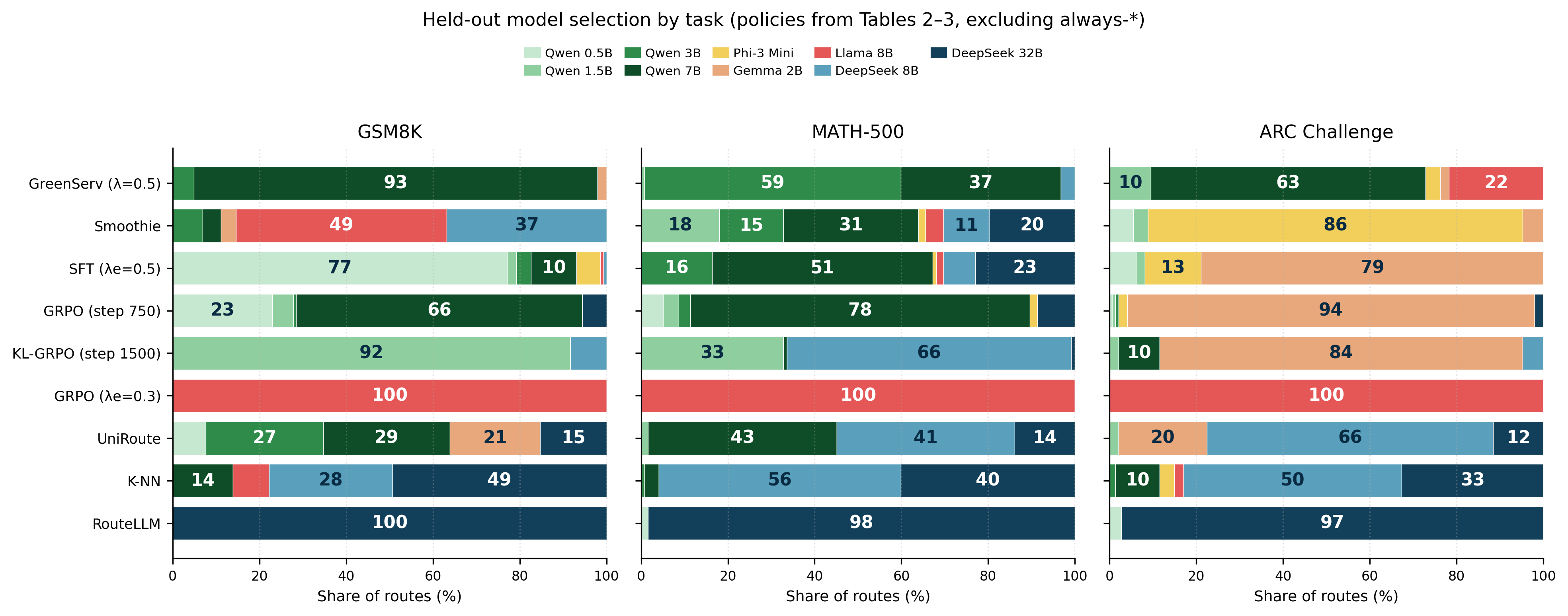
Table 6 orders the TRL sweep by mean answer energy. Matched is cheap and collapsed ( at ). Matched stays below accuracy. The family occupies the mid band. KL-GRPO step 1500 is the highest-accuracy run in that family at and . GRPO step 750 is the cheaper operating point at and . Runs warmed from SFT () jump to about accuracy at more than because that warm start is the accuracy-oracle policy, not a hybrid label set. Table 7 makes the same split at SFT. Hybrid warm starts sit near – and –. SFT () is sft_acc at and .
| Checkpoint | Acc. | Dur. (ms) | Energy (J) | Power (W) |
|---|---|---|---|---|
| GRPO step 1000 (SFT , RL ) | 0.573 | 6002 | 297.0 | 46.8 |
| GRPO step 750 (SFT , RL , run2) | 0.421 | 5634 | 354.7 | 30.4 |
| GRPO step 1000 (SFT , RL , run3) | 0.432 | 6821 | 561.8 | 31.8 |
| GRPO step 1500 (SFT , RL ) | 0.384 | 6070 | 569.3 | 27.9 |
| KL-GRPO step 500 (SFT , RL ) | 0.527 | 7286 | 648.7 | 45.5 |
| KL-GRPO step 1536 (SFT , RL ) | 0.503 | 7410 | 719.2 | 44.4 |
| KL-GRPO step 500 (SFT , RL , choice only) | 0.524 | 7987 | 786.6 | 46.0 |
| GRPO step 750 (SFT , RL , choice only) | 0.584 | 7942 | 811.8 | 48.5 |
| KL-GRPO step 1750 (SFT , RL , choice only) | 0.563 | 8703 | 986.8 | 50.9 |
| KL-GRPO step 500 (SFT , RL ) | 0.549 | 9814 | 1296.8 | 48.6 |
| KL-GRPO step 500 (SFT , RL ) | 0.591 | 10932 | 1339.8 | 47.1 |
| KL-GRPO step 500 (SFT , RL ) | 0.552 | 11809 | 1526.8 | 49.8 |
| GRPO step 1500 (SFT , RL , choice only) | 0.581 | 11860 | 1588.5 | 54.8 |
| GRPO step 1000 (SFT , RL ) | 0.575 | 12561 | 1599.5 | 49.2 |
| KL-GRPO step 1500 (SFT , RL ) | 0.609 | 13118 | 1691.9 | 55.2 |
| GRPO step 1750 (SFT , RL , choice only) | 0.589 | 11764 | 1796.2 | 78.9 |
| GRPO step 1250 (SFT , RL ) | 0.590 | 14076 | 1875.9 | 52.9 |
| GRPO step 2000 (SFT , RL ) | 0.744 | 25574 | 5033.7 | 170.9 |
| GRPO step 1250 (SFT , RL ) | 0.736 | 25581 | 5051.1 | 173.5 |
| GRPO step 500 (SFT , RL ) | 0.738 | 25825 | 5126.7 | 174.2 |
| Checkpoint | Acc. | Dur. (ms) | Energy (J) | Power (W) |
|---|---|---|---|---|
| SFT () | 0.468 | 7517 | 749.9 | 45.5 |
| SFT () | 0.456 | 7588 | 776.7 | 45.0 |
| SFT (, choice only) | 0.544 | 7912 | 779.9 | 47.0 |
| SFT () | 0.502 | 7821 | 822.8 | 45.9 |
| SFT () | 0.738 | 24414 | 4706.6 | 160.3 |
Table 8 is the pool profile that those policies draw from. On held-out testing, Always-Qwen2.5-7B is at , but BBH is only , indicating Qwen2.5-7B’s imbalanced performance across benchmarks. DeepSeek-R1-8B is the strongest overall arm (), but also comes as the expensive always-medium baseline (). DeepSeek-R1-32B is weaker than R1-8B on BBH ( versus ) despite higher energy. Train and held-out accuracy ranks are similar. Train energy is higher because long MATH generations are more common in the train prefix.
| Model | MMLU | GSM8K | BBH | ARC | HellaSwag | MATH-500 | HumanEval | Overall | |
|---|---|---|---|---|---|---|---|---|---|
| Qwen 2.5 0.5B | Acc. | 14.8 | 27.1 | 2.1 | 35.4 | 20.4 | 17.2 | 10.2 | 18.9 |
| Energy | 116.5 | 91.1 | 62.7 | 72.0 | 45.5 | 167.6 | 110.3 | 91.8 | |
| Qwen 2.5 1.5B | Acc. | 37.6 | 59.0 | 8.3 | 68.7 | 44.9 | 32.8 | 30.5 | 41.4 |
| Energy | 126.5 | 129.7 | 84.0 | 92.9 | 66.1 | 226.7 | 105.0 | 117.1 | |
| Qwen 2.5 3B | Acc. | 53.7 | 64.6 | 11.0 | 74.8 | 59.9 | 49.2 | 33.9 | 51.2 |
| Energy | 198.4 | 233.5 | 195.3 | 136.7 | 124.4 | 497.6 | 167.7 | 219.6 | |
| Phi-3 Mini 3.8B | Acc. | 49.0 | 50.0 | 6.2 | 78.9 | 55.1 | 18.0 | 20.3 | 42.2 |
| Energy | 236.1 | 297.0 | 233.8 | 177.5 | 172.3 | 471.4 | 246.7 | 257.8 | |
| Gemma 2 2B | Acc. | 38.3 | 55.6 | 10.3 | 74.8 | 56.5 | 20.5 | 25.4 | 42.2 |
| Energy | 108.5 | 141.3 | 100.6 | 63.2 | 46.4 | 227.1 | 92.1 | 109.9 | |
| Qwen 2.5 7B | Acc. | 59.1 | 84.0 | 26.2 | 84.4 | 61.9 | 67.2 | 67.8 | 64.0 |
| Energy | 219.9 | 311.6 | 263.4 | 149.2 | 141.0 | 701.0 | 221.5 | 281.6 | |
| Llama 3.1 8B | Acc. | 50.3 | 81.2 | 37.9 | 78.9 | 57.8 | 36.9 | 50.8 | 57.3 |
| Energy | 263.4 | 331.9 | 305.8 | 204.4 | 176.6 | 571.4 | 238.0 | 297.0 | |
| DeepSeek-R1 8B | Acc. | 59.7 | 92.4 | 69.7 | 93.2 | 70.7 | 86.1 | 89.8 | 79.1 |
| Energy | 2997.6 | 3318.5 | 3626.6 | 2095.0 | 3744.1 | 8882.8 | 6379.1 | 4127.9 | |
| DeepSeek-R1 32B | Acc. | 65.1 | 89.6 | 27.6 | 92.5 | 72.8 | 86.9 | 94.9 | 73.5 |
| Energy | 3874.6 | 2354.2 | 4403.3 | 3276.1 | 3750.8 | 9080.4 | 16475.5 | 5112.4 |
| Model | MMLU | GSM8K | BBH | ARC | HellaSwag | MATH-500 | HumanEval | Overall | |
|---|---|---|---|---|---|---|---|---|---|
| Qwen 2.5 0.5B | Acc. | 20.9 | 34.5 | 6.8 | 29.5 | 29.5 | 11.7 | 30.0 | 22.5 |
| Energy | 125.8 | 300.7 | 859.4 | 63.4 | 57.6 | 2063.2 | 117.1 | 555.8 | |
| Qwen 2.5 1.5B | Acc. | 42.5 | 61.5 | 18.8 | 65.5 | 40.0 | 32.0 | 64.0 | 44.4 |
| Energy | 151.3 | 888.4 | 803.3 | 80.4 | 72.9 | 2000.3 | 100.8 | 638.5 | |
| Qwen 2.5 3B | Acc. | 45.8 | 52.0 | 23.7 | 71.7 | 56.6 | 46.2 | 52.0 | 49.5 |
| Energy | 203.6 | 250.4 | 698.4 | 129.4 | 135.1 | 1198.4 | 172.6 | 423.1 | |
| Phi-3 Mini 3.8B | Acc. | 41.8 | 58.5 | 16.9 | 80.9 | 55.4 | 11.1 | 30.0 | 43.4 |
| Energy | 249.5 | 1806.7 | 4574.7 | 167.4 | 181.6 | 2971.3 | 238.2 | 1589.2 | |
| Gemma 2 2B | Acc. | 40.9 | 51.7 | 21.2 | 71.1 | 53.5 | 14.8 | 45.0 | 42.3 |
| Energy | 112.5 | 153.5 | 92.3 | 53.1 | 56.2 | 1740.8 | 111.5 | 355.5 | |
| Qwen 2.5 7B | Acc. | 59.4 | 86.2 | 24.6 | 88.3 | 64.6 | 59.4 | 70.0 | 64.0 |
| Energy | 273.4 | 338.7 | 241.0 | 137.0 | 159.4 | 1292.8 | 213.4 | 397.6 | |
| Llama 3.1 8B | Acc. | 43.7 | 76.6 | 40.6 | 80.9 | 55.4 | 31.4 | 56.0 | 54.8 |
| Energy | 336.8 | 1242.2 | 1905.0 | 192.4 | 188.0 | 16106.0 | 223.4 | 3176.9 | |
| DeepSeek-R1 8B | Acc. | 66.8 | 95.1 | 71.4 | 93.2 | 72.9 | 85.8 | 85.0 | 81.1 |
| Energy | 3812.9 | 3586.1 | 5815.8 | 2163.6 | 4468.3 | 13004.1 | 8476.1 | 5621.5 | |
| DeepSeek-R1 32B | Acc. | 70.8 | 94.2 | 32.6 | 94.5 | 69.8 | 79.1 | 93.0 | 74.4 |
| Energy | 4981.8 | 2448.9 | 6337.2 | 3322.3 | 3862.0 | 12974.5 | 13168.3 | 6021.0 |
Figure 10 repeats the four-question layout of Fig. 5 on a later A100-SXM4-GB session using the KL-GRPO step 1500 of a different KL beta variation and the matching SFT eval. The KL-GRPO controller is still about and here about –. SFT is still about and about –. Answer traces for HumanEval q149 and ARC q438 overlap because both policies pick the same model. The large SFT fill is extra controller tokens, not a different GPU. The two figures disagree on absolute watts because board occupancy differed across sessions on the same SKU. Controller energy is therefore a mild add-on to Table 2, not a reason to move the main comparison off answer joules.
