Constrained Flow Policy Updates:
A Generalized Schrödinger Bridge View

Boyang Li Matthew Kim Sylvia Herbert Affiliation: University of California San Diego

Abstract

Online safe reinforcement learning (RL) seeks policies that maximize reward while satisfying safety constraints. Reward and safety can induce multimodal action distributions, challenging the prevailing primal–dual methods: Gaussian actors may collapse onto a single suboptimal mode, and optimization over the nonconvex Lagrangian landscape can be unstable. Diffusion and flow policies can represent such distributions, but recent work with a diffusion actor relies on estimating and matching the score of an augmented-Lagrangian target policy. Instead, we differentiate the augmented objective directly through the generation path of a flow policy, so no score needs to be estimated. Because a flow policy lacks a readily available action log-density for entropy regularization, we build on the density-free kinetic-energy regularizer of FLAC, a recent reward-only method, and propose Reparameterized Augmented-Lagrangian Flow Actor with Least Energy (RAFALE), an off-policy actor–critic method for safe RL. We formulate its update as a constrained one-ended generalized Schrödinger bridge and show that, for each source draw, this path-space problem is exactly an entropy-regularized problem in action space. At positive noise, its solution reweights the reward-only action distribution only where the estimated cost exceeds a threshold set by the Lagrange multiplier. As the noise vanishes, the optimal value converges to that of a least-energy map objective that the flow policy optimizes directly. Across seven Safety-Gymnasium tasks, RAFALE achieves competitive reward with mean final cost within budget on every task, whereas strong baselines trade one for the other; ablations support the necessity of both its augmented objective and its flow actor.

1 Introduction

Safe reinforcement learning (RL) seeks policies that maximize reward while respecting a cost budget. The constrained Markov decision process (CMDP) expresses this requirement as a bound on expected cumulative cost (Altman, 1999; Achiam et al., 2017). Primal–dual methods address it by alternating policy updates with adjustments to a Lagrange multiplier (Stooke et al., 2020), usually with a Gaussian actor. Yet reward and cost can favor separated regions of the action space, producing target distributions that a single Gaussian cannot represent. Moreover, the nonconvex Lagrangian landscape can make primal–dual training unstable (Cheng et al., 2026). Augmented Lagrangian methods address this latter difficulty by modifying the constraint term (Rockafellar, 1973; Bertsekas, 1982; Wu et al., 2024).

Diffusion and flow policies are expressive enough to represent such distributions in online RL. The methods that train them differ in how the critic enters generation (Gao et al., 2026): 1) Q-value guidance matches the score network to the critic’s action gradient (Psenka et al., 2024); 2) weighted matching regresses the model onto a score estimated from critic-weighted samples (Ma et al., 2025; Li et al., 2026b; Kim et al., 2026; Ma et al., 2026); 3) policy-gradient methods optimize an on-policy surrogate (McAllister et al., 2026; Yi et al., 2026); and 4) reparameterization differentiates the critic through the sampler (Wang et al., 2024; Celik et al., 2025; Lv et al., 2026). Related safe RL methods with generative policies use the first two approaches: score-based updates. Offline, FISOR extracts a diffusion policy by feasibility-guided weighted regression (Zheng et al., 2024). Online, ALGD trains a diffusion policy to match an estimated score of the Boltzmann policy whose energy is the augmented Lagrangian (Cheng et al., 2026).

A direct update would avoid estimating a score altogether. Reparameterization provides one for Gaussian actors, which are updated from the pathwise gradient of the critic at the generated action. For diffusion and flow policies, however, such an update is harder to regularize. Exploration requires the policy to remain stochastic (Ziebart, 2010; Haarnoja et al., 2018), but the usual entropy term needs an action log-density that these samplers do not readily provide. Reward-only methods therefore estimate the entropy along the sampling chain (Celik et al., 2025) or regularize a tractable proxy (Wang et al., 2024). FLAC offers a promising alternative for reward maximization: it regularizes the generation process in path space, keeping it close to a high-entropy reference process through a one-ended generalized Schrödinger bridge (Lv et al., 2026). This yields a density-free kinetic-energy regularizer. For safe RL, three questions remain: what this path-space regularization does to the action distribution, how the constraint reshapes that distribution, and how it relates to the deterministic flow update used in training.

Building on FLAC, we propose Reparameterized Augmented-Lagrangian Flow Actor with Least Energy (RAFALE). It evaluates the augmented Lagrangian at the generated action and differentiates it through the flow, so the constraint reaches the policy through a pathwise gradient rather than an estimated score. We answer the three questions through a constrained one-ended Schrödinger bridge. Our central observation is that, for each source draw, this path-space problem is exactly an entropy-regularized problem in action space. Keeping the generation process close to Brownian motion balances the augmented Lagrangian plus a displacement from the source draw against the entropy of the action distribution, so the solution becomes a Gibbs distribution. The constraint reweights this distribution: actions whose estimated cost exceeds a threshold set by the multiplier are downweighted increasingly with that cost, while the relative probabilities of the remaining actions are unchanged. The vanishing-noise limit of this problem gives a deterministic-map objective whose restriction to a midpoint sampler is exactly the actor loss of RAFALE.

Table 1: Positioning by setting, actor class, constraint type, and actor-update route; a related taxonomy appears in Gao et al. (2026). RAFALE occupies the online, constrained, generative-policy, reparameterization cell.

Method	Setting	Actor	Constraint	Actor update
PID-Lag (Stooke et al., 2020)	online	Gaussian	expected cost	policy gradient
CAL (Wu et al., 2024)	online	Gaussian	expected cost	reparameterization
RCRL (Yu et al., 2022)	online	Gaussian	state-wise	reparameterization
RESPO (Ganai et al., 2023)	online	Gaussian	state-wise	policy gradient
QSM (Psenka et al., 2024)	online	diffusion	none	Q-value guidance
RSM, RFM, FLAG (Ma et al., 2025; Li et al., 2026b; Kim et al., 2026)	online	diffusion, flow	none	weighted matching
FPO (McAllister et al., 2026)	online	flow	none	policy gradient
DACER, DIME (Wang et al., 2024; Celik et al., 2025)	online	diffusion	none	reparameterization
FLAC (Lv et al., 2026)	online	flow	none	reparameterization
FISOR (Zheng et al., 2024)	offline	diffusion	state-wise	weighted matching
ALGD (Cheng et al., 2026)	online	diffusion	expected cost	Q-value guidance
RAFALE (ours)	online	flow	expected cost	reparameterization

Our contributions are threefold:

•

A constrained Schrödinger-bridge analysis of flow updates. We show that, for each source draw, the constrained one-ended Schrödinger bridge is an entropy-regularized problem in action space. We then characterize its Gibbs solution and safety tilt and derive its vanishing-noise map objective (Section 4).
•

A direct flow-policy algorithm. RAFALE optimizes the map objective through a midpoint sampler, combining the constraint term with kinetic regularization and off-policy critic learning (Section 5).
•

Evaluation in online safe RL. On seven Safety-Gymnasium tasks, RAFALE achieves competitive reward with mean final cost within budget on every task. Ablations compare the augmented objective with standard and hinge alternatives, and the flow actor with Gaussian and mixture actors (Section 6).

2 Related Work

Due to space limits, we discuss here only the work closest to RAFALE; Appendix A describes the four routes of Section 1 and safe RL with generative actors in detail. RAFALE follows the fourth route, and Table 1 places representative methods of each route by setting, actor class, and constraint type.

Within safe RL, CAL applies an augmented Lagrangian to a policy-level expected constraint residual with a Gaussian actor (Wu et al., 2024). ALGD applies it at the action level and, following the first route, estimates the noisy-time score of the resulting Boltzmann policy for a diffusion actor (Cheng et al., 2026). We retain the action-level objective but optimize it through a flow sampler, along the fourth route. This expected-cost formulation differs from the state-wise reachability constraints used by RCRL and RESPO (Yu et al., 2022; Ganai et al., 2023) and by the offline generative methods FISOR and EpiFlow (Zheng et al., 2024; Tayal & Tayal, 2026).

KL control and Schrödinger bridges provide the basis for our reference-process regularizer (Todorov, 2006; Léonard, 2014; Chen et al., 2016; Zhang & Chen, 2022; Liu et al., 2024). FLAC derives kinetic-energy regularization from this perspective for reward-only flow policies (Lv et al., 2026), and SoftGAC decomposes a path-space regularizer at the endpoint for a reward-only bridge actor (He et al., 2026). We extend this analysis to the augmented Lagrangian: with a Brownian reference, the endpoint term becomes a displacement plus a conditional entropy, and the noise-free limit gives the objective of a deterministic flow actor.

3 The Constrained Flow-Update Problem

3.1 From an Episodic Constraint to an Actor Objective

We consider a CMDP $(\mathcal{S},\mathcal{A},p,d_{0},r,c,\gamma,H)$ , where $\mathcal{S}$ and $\mathcal{A}$ are continuous state and action spaces, $p$ is the transition kernel, and $d_{0}$ is the initial-state distribution. The reward $r$ , nonnegative cost $c$ , discount $\gamma\in(0,1)$ , and episode horizon $H$ define the objective

\max_{\pi}\;J_{r}(\pi):=\mathbb{E}_{\pi}\Big[\sum_{k<H}\gamma^{k}r(s_{k},a_{k})\Big]\quad\text{s.t.}\quad J_{c}(\pi):=\mathbb{E}_{\pi}\Big[\sum_{k<H}c(s_{k},a_{k})\Big]\leq b,

(1)

where $s_{0}\sim d_{0}$ , $a_{k}\sim\pi(\cdot\mid s_{k})$ , and $s_{k+1}\sim p(\cdot\mid s_{k},a_{k})$ . The budget $b$ thus limits the expected undiscounted cost of an episode rather than the cost at every state.

Although Equation 1 evaluates complete episodes, the actor must compare individual actions. Reward and cost action values make this comparison possible by accounting for what follows each action under the current policy:

Q_{x}(s,a):=\mathbb{E}_{\pi}\Big[\sum_{k\geq 0}\gamma^{k}x(s_{k},a_{k})\,\Big|\,s_{0}=s,\ a_{0}=a\Big],\qquad x\in\{r,c\}.

(2)

We estimate these values with off-policy critics trained on replay data (Liu et al., 2022; Wu et al., 2024). Since $Q_{c}$ is discounted while the episode budget is not, we use a nominal budget $h$ in critic units, converted as specified in Appendix D. Following primal–dual methods (Altman, 1999; Achiam et al., 2017; Stooke et al., 2020), we combine the two critics with a nonnegative multiplier $\lambda$ . For given critics and multiplier, the standard action-level Lagrangian is

L(s,a):=-Q_{r}(s,a)+\lambda\,\big(Q_{c}(s,a)-h\big).

(3)

Minimizing its expectation favors higher reward while accounting for future cost, with $\lambda$ setting the relative weight of the two objectives.

Primal–dual updates built on $L$ , however, are prone to oscillation: the multiplier integrates past constraint violations, which makes the cost oscillate around the budget (Stooke et al., 2020). The augmented Lagrangian is the classical remedy, because it smooths the dual problem (Rockafellar, 1973; Rockafellar, 1976; Bertsekas, 1982), and Cheng et al. (2026) analyze its effect on the action-level landscape of a generative actor. At the action level, it replaces the linear constraint term of $L$ by a piecewise quadratic one:

L_{A}(s,a):=-Q_{r}(s,a)+\Phi_{\lambda,\rho}\big(Q_{c}(s,a)-h\big),\qquad\Phi_{\lambda,\rho}(y):=\frac{[\lambda+\rho y]_{+}^{2}-\lambda^{2}}{2\rho},

(4)

where $[y]_{+}=\max\{y,0\}$ and $\rho>0$ sets the strength of the quadratic part. To see which actions this term affects, we rewrite it around the activation threshold $\tau$ :

L_{A}(s,a)=-Q_{r}(s,a)+\frac{\rho}{2}\big[Q_{c}(s,a)-\tau\big]_{+}^{2}-\frac{\lambda^{2}}{2\rho},\qquad\tau:=h-\lambda/\rho.

(5)

Below $\tau$ , $L_{A}$ differs from $-Q_{r}$ only by an action-independent constant. Above $\tau$ , the added term grows quadratically with the excess of the estimated cost over $\tau$ , which is the active-set structure of the augmented Lagrangian (Hintermüller & Kunisch, 2006). The multiplier determines where this influence begins: $\tau$ lies below the nominal budget $h$ whenever $\lambda>0$ , and a larger $\lambda$ lowers it further, enlarging the set of actions on which the constraint term acts.

3.2 A Direct Actor Update for a Flow Policy

The objective $L_{A}$ tells us how to compare actions, but learning a policy also requires a way to transmit this objective to the actor. A flow policy provides a differentiable generation process: a source sample $x_{0}\sim\mu_{0}$ evolves under a state-conditioned velocity field,

\frac{dX_{t}}{dt}=v(s,X_{t},t),\qquad X_{0}=x_{0},\qquad t\in[0,1].

(6)

At a fixed state $s$ , a numerical solver produces the endpoint $a:=X_{1}$ (Lipman et al., 2023).¹¹ 1 For bounded environment actions, $X_{1}$ is the unsquashed output, and critic evaluations include the final tanh map. Kinetic energy is measured before squashing; see Appendix D. Each source draw gives a deterministic endpoint, while sampling $x_{0}$ induces the policy distribution. Because the solver is differentiable, the critic can update this generator through the action it produces. We therefore evaluate $L_{A}$ at the endpoint and optimize its expectation, extending the reparameterized updates of reward-only generative policies (Wang et al., 2024; Celik et al., 2025; Lv et al., 2026):

Problem 1 (Direct constrained flow update).

\min_{v}\;\mathbb{E}_{s\sim\mathcal{D},\,x_{0}\sim\mu_{0}}\big[L_{A}\big(s,X_{1}\big)\big],

(7)

where $s\sim\mathcal{D}$ denotes sampling states from the replay buffer. The constraint thus reaches the actor through the same pathwise derivative as the reward term, without an intermediate score estimate. Problem 1, however, contains no entropy regularization. Its minimizers do not depend on $x_{0}$ , so the update can map every source draw to the same minimizer of $L_{A}$ , and the policy may collapse prematurely and stop exploring.

4 A Safety-Tilted Schrödinger Bridge

Maximum-entropy RL avoids this collapse through entropy regularization, which requires an action log-density that our flow sampler does not readily provide (Haarnoja et al., 2018). Following FLAC (Lv et al., 2026), we therefore regularize the generation process in path space, where the regularizer needs no action log-density, instead of the action distribution in action space. The central result of this section is that, for each source draw, this path-space regularization is exactly an entropy-regularized problem in action space (Theorem 1); its solution and noise-free limit then determine the update of RAFALE.

4.1 From a Reference Process to Kinetic Regularization

We take as the reference a zero-drift Brownian process, which adds isotropic noise to each source draw:

dX_{t}=\sqrt{\varepsilon}\,dW_{t},\qquad X_{0}\sim\mu_{0},\qquad t\in[0,1],

(8)

where $W$ is a standard Brownian motion and $\varepsilon>0$ . We write $R^{\varepsilon}$ for its path distribution and $R_{1}^{\varepsilon}$ for the distribution of its endpoint $X_{1}$ , which is the source distribution spread by Gaussian noise of variance $\varepsilon$ . The desired generation process starts from $\mu_{0}$ , ends at actions with low $L_{A}$ , and stays close to $R^{\varepsilon}$ . The following problem formalizes this trade-off in path space:

Problem 2 (Constrained one-ended Schrödinger bridge).

\mathcal{B}^{\varepsilon}(s):=\inf_{P:\,P_{0}=\mu_{0}}\Big\{\mathbb{E}_{P}\big[L_{A}(s,X_{1})\big]+\alpha\varepsilon\,D_{\mathrm{KL}}(P\|R^{\varepsilon})\Big\},\qquad\alpha>0.

(9)

Problem 2 is a one-ended generalized Schrödinger bridge (Todorov, 2006; Zhang & Chen, 2022; Liu et al., 2024). Unlike a classical Schrödinger bridge, it fixes only the source distribution $P_{0}=\mu_{0}$ and leaves the action distribution $P_{1}$ free, since we have no target action distribution to match. Following FLAC (Lv et al., 2026), we call $L_{A}$ , which shapes $P_{1}$ , the terminal potential.

Problem 2, however, cannot be optimized with our sampler as written. Its KL term is defined by the density ratio $dP/dR^{\varepsilon}$ between path distributions, whereas the sampler only generates paths from a velocity field. We therefore express the KL through that field. Let the generation process follow a velocity field $v$ under the reference noise,

dX_{t}=v(s,X_{t},t)\,dt+\sqrt{\varepsilon}\,dW_{t},\qquad X_{0}\sim\mu_{0},\qquad t\in[0,1],

(10)

and let $P$ denote its path distribution. Because Equation 10 and Equation 8 share the noise, Girsanov’s theorem (Léonard, 2014) gives

\varepsilon\,D_{\mathrm{KL}}(P\|R^{\varepsilon})=\frac{1}{2}\,\mathbb{E}_{P}\Big[\int_{0}^{1}\|v(s,X_{t},t)\|^{2}\,dt\Big]

(11)

under the conditions of Section B.1. Scaled by $\varepsilon$ , the divergence from the reference is thus the expected kinetic energy of the drift. Substituting it into Problem 2 gives an equivalent reformulation over velocity fields, with the same value and the same optimal path distribution (Section B.1):

Problem 3 (Equivalent kinetic-energy reformulation).

\mathcal{B}^{\varepsilon}(s)=\inf_{v}\;\mathbb{E}\Big[L_{A}(s,X_{1})+\frac{\alpha}{2}\int_{0}^{1}\|v(s,X_{t},t)\|^{2}\,dt\Big],\qquad X\text{ follows \lx@cref{creftype~refnum}{eq:controlled}}.

(12)

Both terms of its objective can be estimated from generated paths: the terminal potential from the critics at $X_{1}$ , and the kinetic energy from the velocities along the path. Unlike Problem 2, Problem 3 thus requires no density ratio; Section 4.3 connects it to the deterministic sampler of RAFALE.

The kinetic energy also controls the action distribution. Since the endpoint $X_{1}$ is a function of the path, the data-processing inequality bounds the divergence between endpoint distributions by the divergence between path distributions (Section B.1), and Equation 11 turns the latter into kinetic energy:

D_{\mathrm{KL}}(P_{1}\|R_{1}^{\varepsilon})\;\leq\;D_{\mathrm{KL}}(P\|R^{\varepsilon})=\frac{1}{2\varepsilon}\,\mathbb{E}_{P}\Big[\int_{0}^{1}\|v(s,X_{t},t)\|^{2}\,dt\Big].

(13)

Minimizing the kinetic energy thus keeps the action distribution $P_{1}$ close to the broad reference distribution $R_{1}^{\varepsilon}$ without evaluating its density.

4.2 Action-Space Form and Safety Tilt

The bound of Equation 13 limits the divergence of the action distribution, but it does not reveal which action distribution Problem 3 selects. The next result answers this exactly: for each source draw, the path-space problem is an entropy-regularized problem in action space, which yields both the solution and its noise-free limit.

Theorem 1 (Action-space form).

Let $\varepsilon>0$ . Under the conditions of Section B.1, Problems 2 and 3 are equivalent to the following problem over conditional action distributions:

\mathcal{B}^{\varepsilon}(s)=\mathbb{E}_{x_{0}\sim\mu_{0}}\Big[\min_{q}\Big\{\mathbb{E}_{a\sim q}\big[L_{A}(s,a)+\alpha\,\mathcal{E}(x_{0},a)\big]-\alpha\varepsilon\,H(q)\Big\}\Big]+\frac{\alpha\varepsilon d_{a}}{2}\log(2\pi\varepsilon).

(14)

Here $q$ ranges over densities of actions, $\mathcal{E}(x_{0},a):=\tfrac{1}{2}\|a-x_{0}\|^{2}$ , $H(q):=-\int q(a)\log q(a)\,da$ , and $d_{a}$ is the action dimension. An optimal generation process draws its action from the minimizer in Equation 14 and connects each source draw to its action by a Brownian bridge.

We prove Theorem 1 in Section B.1 from the chain rule for the KL divergence and the Gaussian endpoint $\mathcal{N}(x_{0},\varepsilon I)$ of the reference. It is the static form of the Schrödinger problem (Léonard, 2014), written for our one-ended setting. The theorem connects the path-space view of regularization, taken by FLAC, with the action-space view of maximum-entropy RL. For each source draw, the KL to the reference acts on the actions through two terms. The displacement $\mathcal{E}(x_{0},a)$ is the kinetic energy of the straight path from $x_{0}$ to $a$ at constant speed. The sum $L_{A}+\alpha\mathcal{E}$ is therefore the total energy of reaching $a$ : the terminal potential plus $\alpha$ times this kinetic energy. The entropy $H(q)$ , conditional on the source draw and weighted by the temperature $\alpha\varepsilon$ , spreads the actions. Keeping the generation process close to Brownian motion is therefore exactly entropy regularization of the actions generated from each source draw, anchored to that draw by the displacement. The constant in Equation 14 does not depend on $q$ .

Because Equation 14 is entropy-regularized, its minimizer is a Boltzmann distribution. Theorem 2 gives this minimizer and compares it with the reward-only Schrödinger bridge of FLAC, obtained by replacing $L_{A}$ with $-Q_{r}$ , to isolate the effect of the constraint.

Theorem 2 (Gibbs solution and safety tilt).

Let $\varepsilon>0$ . Let $q_{A}^{\varepsilon}(\cdot\mid s,x_{0})$ denote the minimizer in Equation 14, and let $q_{R}^{\varepsilon}(\cdot\mid s,x_{0})$ denote the minimizer when $L_{A}$ is replaced by $-Q_{r}$ . Under the conditions of Section B.1:

(a) Gibbs solution.

	$\displaystyle q_{R}^{\varepsilon}(a\mid s,x_{0})$	$\displaystyle\propto\exp\Big\{-\frac{-Q_{r}(s,a)+\alpha\,\mathcal{E}(x_{0},a)}{\alpha\varepsilon}\Big\},$
	$\displaystyle q_{A}^{\varepsilon}(a\mid s,x_{0})$	$\displaystyle\propto\exp\Big\{-\frac{L_{A}(s,a)+\alpha\,\mathcal{E}(x_{0},a)}{\alpha\varepsilon}\Big\}.$		(15)

(b) Safety tilt. The two densities satisfy

	$\displaystyle q_{A}^{\varepsilon}(a\mid s,x_{0})$	$\displaystyle=q_{R}^{\varepsilon}(a\mid s,x_{0})\,\frac{w^{\varepsilon}(s,a)}{Z^{\varepsilon}(s,x_{0})},\qquad w^{\varepsilon}(s,a):=\exp\!\Big[-\frac{\rho}{2\alpha\varepsilon}\big[Q_{c}(s,a)-\tau\big]_{+}^{2}\Big],$		(16)
	$\displaystyle Z^{\varepsilon}(s,x_{0})$	$\displaystyle:=\mathbb{E}_{a^{\prime}\sim q_{R}^{\varepsilon}(\cdot\mid s,x_{0})}\big[w^{\varepsilon}(s,a^{\prime})\big]\leq 1.$

Part (a) follows from Equation 14 by the Gibbs variational principle (Section B.1). The solution compares two actions $a$ and $a^{\prime}$ generated from the same source draw through their total energy alone:

\frac{q_{A}^{\varepsilon}(a\mid s,x_{0})}{q_{A}^{\varepsilon}(a^{\prime}\mid s,x_{0})}=\exp\Big\{-\frac{\big[L_{A}(s,a)-L_{A}(s,a^{\prime})\big]+\alpha\big[\mathcal{E}(x_{0},a)-\mathcal{E}(x_{0},a^{\prime})\big]}{\alpha\varepsilon}\Big\}.

(17)

An action is thus more likely when it lowers $L_{A}$ by more than $\alpha$ times its extra displacement.

Part (b) isolates the effect of the constraint. The normalizer $Z^{\varepsilon}(s,x_{0})$ depends only on the source draw, so it cancels when two actions from the same source draw are compared, and Equation 16 gives

\frac{q_{A}^{\varepsilon}(a\mid s,x_{0})}{q_{A}^{\varepsilon}(a^{\prime}\mid s,x_{0})}=\frac{q_{R}^{\varepsilon}(a\mid s,x_{0})}{q_{R}^{\varepsilon}(a^{\prime}\mid s,x_{0})}\cdot\frac{w^{\varepsilon}(s,a)}{w^{\varepsilon}(s,a^{\prime})}.

(18)

If both actions satisfy $Q_{c}\leq\tau$ , both weights equal one and the reward-only ratio is unchanged. Otherwise, the action with the higher estimated cost above $\tau$ becomes less likely to be selected relative to the other, increasingly with that cost. The constraint therefore lowers the probability of selecting actions with high estimated cost (Section B.3).

4.3 The Vanishing-Noise Limit

Theorems 1 and 2 characterize the Schrödinger bridge at positive noise, whereas the actor of RAFALE is a deterministic flow, which sends each source draw to a single action. We therefore study the limit of Problem 3, equivalently of Equation 14, as $\varepsilon\to 0$ with $\alpha$ fixed. In Equation 14, this limit removes only the entropy term and the constant, so each conditional solution concentrates on the minimizers of the total energy $L_{A}+\alpha\mathcal{E}$ . Theorem 3 makes this precise.

Theorem 3 (Vanishing noise).

Under the conditions of Section B.1, for each state $s$ ,

\lim_{\varepsilon\downarrow 0}\mathcal{B}^{\varepsilon}(s)=\inf_{T}\;\mathbb{E}_{x_{0}\sim\mu_{0}}\Big[L_{A}\big(s,T(x_{0})\big)+\alpha\,\mathcal{E}\big(x_{0},T(x_{0})\big)\Big],

(19)

where $T$ ranges over the square-integrable maps $L^{2}(\mu_{0};\mathbb{R}^{d_{a}})$ from source draws to actions and $d_{a}$ is the action dimension. The infimum is attained, and $T$ attains it if and only if, for $\mu_{0}$ -almost every $x_{0}$ ,

T(x_{0})\in\operatorname*{arg\,min}_{a}\,\big\{L_{A}(s,a)+\alpha\,\mathcal{E}(x_{0},a)\big\}.

(20)

Without noise, Problem 3 thus reduces to choosing one action per source draw: its value converges to that of Equation 19, and an optimal map sends each source draw to a minimizer of its total energy.

The limit does not remove the randomness of the policy. The positive-noise solution of Equation 14 is random for two reasons: the source draw $x_{0}$ is random, and, given $x_{0}$ , the entropy term spreads the actions. The limit problem of Theorem 3 removes only the second. The first remains because the displacement makes the minimizer in Equation 20 depend on $x_{0}$ : for differentiable $L_{A}$ , the optimal map sends distinct source draws to distinct actions (Sections B.5 and C). The minimizers of Problem 1, by contrast, do not depend on $x_{0}$ , so Problem 1 can send every source draw to the same action (Section 3.2). In the noise-free limit, the kinetic regularization thus acts through the source draws, geometrically, rather than through the entropy of each conditional distribution.

5 Practical Online Algorithm

RAFALE minimizes the objective of Theorem 3, the noise-free limit of the action-space problem Equation 14, over maps given by a velocity network $v_{\theta}$ and one explicit midpoint step. The step, which FLAC also uses, requires two network evaluations:

X_{1}=x_{0}+\delta_{\theta}(s,x_{0}),\qquad\delta_{\theta}(s,x_{0})=v_{\theta}\!\left(s,x_{0}+\tfrac{1}{2}v_{\theta}(s,x_{0},0),\tfrac{1}{2}\right).

(21)

The same evaluations give the kinetic energy of the step,

K_{\theta}(s,x_{0}):=\tfrac{1}{2}\|\delta_{\theta}(s,x_{0})\|^{2}=\tfrac{1}{2}\|X_{1}-x_{0}\|^{2}=\mathcal{E}(x_{0},X_{1}),

(22)

which is exactly the displacement $\mathcal{E}(x_{0},X_{1})$ of Theorem 3, so the one-step sampler evaluates the regularizer of the limit objective without approximation. Evaluating Equation 19 at the midpoint map and averaging over replay states therefore gives the actor loss (Section B.2):

\mathcal{L}(\theta):=\mathbb{E}_{s\sim\mathcal{D},\,x_{0}\sim\mu_{0}}\Big[-Q_{r}(s,X_{1})+\Phi_{\lambda,\rho}\big(Q_{c}(s,X_{1})-h\big)+\alpha K_{\theta}(s,x_{0})\Big].

(23)

We estimate the loss with one source draw per replay state and backpropagate through both velocity evaluations, so neither the Gibbs density of Theorem 2 nor its score is estimated during training.

To use Equation 23 online, we learn its critics from replay and adjust the multiplier using completed episodes; Algorithm 1 in Appendix D summarizes the learner. Two reward critics use clipped double Q-learning (Fujimoto et al., 2018), with their minimum supplying $Q_{r}$ , alongside a single cost critic $Q_{c}$ . Following FLAC (Lv et al., 2026), the reward backup subtracts $\alpha$ times the kinetic energy of the next action, so $Q_{r}$ is a kinetic-energy-regularized reward critic. The multiplier instead follows a projected proportional–integral rule driven by measured episode costs (Stooke et al., 2020). Data collection and evaluation use the same midpoint sampler, without candidate selection.

Kinetic-energy adaptation.

Because kinetic energy varies across tasks and training stages, a fixed $\alpha$ can constrain the generator too strongly or too weakly. We therefore use the automatic tuning rule of FLAC, updating $\log\alpha$ by gradient descent on

\mathcal{L}_{\alpha}=\log\alpha\,\big(K_{\mathrm{tgt}}-\operatorname{stopgrad}(\widehat{K})\big),\qquad K_{\mathrm{tgt}}=1.125\,d_{a},

(24)

where $\widehat{K}$ is the minibatch mean kinetic energy and $d_{a}$ is the action dimension. Energy above the target increases $\alpha$ and strengthens the regularizer, while energy below it decreases $\alpha$ .

Table 2: Final episodic reward and cost (mean

\pm

SD, five seeds;

b=10

, or

25

on CarGoal); RESPO trains for 9M–10M environment steps, the others for 1M–3M (Appendix E). Red: mean cost above budget. Among entries within budget, bold blue and bold green mark the highest and second-highest reward.

Task	Metric	RESPO	CAL	RCRL	ALGD	RAFALE (ours)
Swimmer	Reward	$36\pm 3$	$41\pm 3$	$20\pm 15$	$\bm{52\pm 13}$	$\bm{93\pm 23}$
Swimmer	Cost	$7.5\pm 0.6$	$16.6\pm 6.7$	$4.0\pm 7.6$	$2.9\pm 3.5$	$5.4\pm 2.7$
HalfCheetah	Reward	$\bm{2344\pm 320}$	$2650\pm 111$	$1796\pm 2493$	$2817\pm 69$	$\bm{3025\pm 55}$
HalfCheetah	Cost	$9.8\pm 5.9$	$15.5\pm 14.7$	$195.2\pm 434.8$	$22.4\pm 44.7$	$3.5\pm 4.7$
Hopper	Reward	$\bm{1073\pm 308}$	$1664\pm 24$	$1037\pm 575$	$1702\pm 15$	$\bm{1655\pm 46}$
Hopper	Cost	$3.1\pm 5.1$	$12.2\pm 6.2$	$0.2\pm 0.3$	$15.7\pm 12.3$	$0.3\pm 0.4$
Walker2d	Reward	$2925\pm 66$	$\bm{2894\pm 56}$	$1758\pm 871$	$2920\pm 133$	$\bm{3177\pm 26}$
Walker2d	Cost	$10.6\pm 3.2$	$6.3\pm 3.8$	$10.1\pm 16.0$	$17.1\pm 15.2$	$1.3\pm 1.3$
Ant	Reward	$\bm{1950\pm 75}$	$2815\pm 265$	$2332\pm 1292$	$2218\pm 1735$	$\bm{3427\pm 62}$
Ant	Cost	$5.6\pm 1.1$	$11.1\pm 9.4$	$76.3\pm 169.7$	$16.8\pm 11.9$	$4.4\pm 1.7$
Humanoid	Reward	$\bm{5380\pm 900}$	$5289\pm 167$	$5640\pm 705$	$4530\pm 829$	$\bm{6513\pm 27}$
Humanoid	Cost	$1.5\pm 1.1$	$0.1\pm 0.2$	$15.2\pm 34.0$	$0.2\pm 0.5$	$3.2\pm 3.1$
CarGoal	Reward	$\bm{20.0\pm 1.3}$	$12.1\pm 1.7$	$1.2\pm 0.8$	$16.5\pm 2.6$	$\bm{18.3\pm 1.6}$
CarGoal	Cost	$20.8\pm 3.9$	$12.3\pm 2.6$	$26.1\pm 11.6$	$22.4\pm 4.8$	$20.7\pm 3.3$
Tasks within budget		6/7	3/7	2/7	3/7	7/7

Figure 1: Learning curves (mean

\pm 1

standard error over five seeds): test reward (upper rows) and test cost (lower rows) against environment steps. Dashed lines mark the budget, and cost axes are truncated. RESPO, trained for up to 10M steps, appears in Figure 2.

6 Experiments

We test RAFALE on six velocity-constrained locomotion tasks and the navigation task CarGoal from Safety-Gymnasium (Ji et al., 2023). The episodic cost budget is $b=10$ for locomotion and $b=25$ for CarGoal. We report final-policy reward and cost as mean $\pm$ standard deviation over five seeds; a run is feasible when its mean evaluation cost is at most $b$ . All methods are evaluated at a fixed endpoint checkpoint (Appendix E).

Baselines.

CAL (Wu et al., 2024) and ALGD (Cheng et al., 2026) are off-policy primal–dual baselines with Gaussian and diffusion actors. RCRL (Yu et al., 2022) and RESPO (Ganai et al., 2023) instead use state-wise reachability constraints, a stricter safety objective than an expected-cost budget; RCRL is off-policy, and RESPO is on-policy with substantially more environment steps.

6.1 Main Results

RAFALE is the only method with mean final cost within budget on every task (Table 2). Among the entries within budget, it has the highest reward on all locomotion tasks, and RESPO has the highest reward on CarGoal. CAL and ALGD attain competitive reward, but each exceeds the budget on more than half of the tasks. The reachability-based methods obtain lower reward on locomotion, even with the longer training schedule of RESPO; RESPO is feasible on nearly every task, whereas RCRL exceeds the budget on most of them. Figure 1 also shows transient cost excursions during training (Section 7).

6.2 Ablation Studies

We ablate both components on Hopper, Walker2d, and Humanoid (protocols in Section E.4).

Augmented versus standard Lagrangian.

To separate activation at a threshold from growth above it, we compare $L_{A}$ with the standard Lagrangian $L$ and a hinge control $L_{C}:=-Q_{r}+\lambda[Q_{c}-\tau]_{+}$ , which keeps the threshold of $L_{A}$ but grows linearly above it. All other learner settings, including the multiplier update rule, are shared. On Hopper and Walker2d, the augmented objective gives higher final reward and lower peak and integrated excess of evaluated cost (Table 3). On Humanoid, final reward and integrated excess are similar, but the augmented objective is the only variant whose five final runs are all feasible. The hinge variant has a higher peak cost on every task, which suggests that the improvement depends on how the constraint term grows above the threshold, not only on the threshold itself.

Effect of the actor family.

To compare actor families under the same constraint mechanism, we replace the flow actor with tanh-Gaussian and eight-component tanh-GMM actors, each trained with its native regularizer, and leave the remaining settings unchanged. The flow actor attains the lowest mean final cost on all three tasks with comparable reward (Table 4), although its cost advantage over the GMM is small on Walker2d. Only the flow configuration has feasible final policies in every run, so the flow actor satisfies the budget more reliably without sacrificing reward.

Table 3: Lagrangian ablation (five seeds; mean

\pm

SD where shown): final reward and cost, peak evaluated cost (Peak), integrated excess above budget (Excess), and feasible final seeds (Feas.). Bold blue: highest reward; bold black: lowest Peak and Excess, most feasible seeds.

Task	Variant	Reward	Cost	Peak	Excess	Feas.
Hopper	Augmented $A$ (RAFALE)	$\bm{1655\pm 46}$	$0.3\pm 0.4$	$\bm{174.6}$	$\bm{92.3\pm 15.9}$	5/5
	Hinge $C$	$1547\pm 33$	$0.8\pm 1.2$	902.9	$251.2\pm 30.3$	5/5
	Standard $U$	$1208\pm 573$	$0.0\pm 0.1$	767.8	$240.6\pm 70.2$	5/5
Walker2d	Augmented $A$ (RAFALE)	$\bm{3177\pm 26}$	$1.3\pm 1.3$	$\bm{125.9}$	$\bm{20.3\pm 3.8}$	5/5
	Hinge $C$	$3075\pm 89$	$0.0\pm 0.0$	390.1	$55.9\pm 28.4$	5/5
	Standard $U$	$2939\pm 65$	$1.2\pm 2.1$	443.8	$83.7\pm 42.9$	5/5
Humanoid	Augmented $A$ (RAFALE)	$6513\pm 27$	$3.2\pm 3.1$	$\bm{81.8}$	$32.3\pm 7.7$	5/5
	Hinge $C$	$6540\pm 28$	$9.1\pm 4.3$	128.9	$32.3\pm 12.1$	3/5
	Standard $U$	$\bm{6543\pm 11}$	$8.0\pm 13.9$	147.3	$33.7\pm 12.7$	4/5

Table 4: Actor families with their native regularizers: final reward / cost (mean

\pm

SD, five seeds; feasible seeds in parentheses). Bold blue: highest reward; bold black: lowest cost.

Task	Flow (RAFALE)	Gaussian	GMM
Hopper	${\color[rgb]{0,0.2734,0.6602}\bm{1655\!\pm\!46}}\;/\;\bm{0.3\!\pm\!0.4}$ (5)	$1408\!\pm\!506\;/\;7.6\!\pm\!17.0$ (4)	$1645\!\pm\!51\;/\;1.5\!\pm\!2.4$ (5)
Walker2d	$3177\!\pm\!26\;/\;\bm{1.3\!\pm\!1.3}$ (5)	$3151\!\pm\!15\;/\;3.5\!\pm\!4.0$ (4)	${\color[rgb]{0,0.2734,0.6602}\bm{3190\!\pm\!17}}\;/\;1.4\!\pm\!1.1$ (5)
Humanoid	${\color[rgb]{0,0.2734,0.6602}\bm{6513\!\pm\!27}}\;/\;\bm{3.2\!\pm\!3.1}$ (5)	$6510\!\pm\!51\;/\;8.1\!\pm\!2.6$ (4)	$6503\!\pm\!116\;/\;8.5\!\pm\!5.1$ (3)

7 Conclusion and Limitations

We introduced RAFALE by formulating a constrained flow update as a one-ended Schrödinger bridge, whose reference-process regularizer becomes a computable kinetic-energy term. Our analysis shows that, for each source draw, this path-space problem is exactly an entropy-regularized problem in action space. Its Gibbs solution lowers the probability of actions whose estimated cost exceeds a threshold set by the multiplier, and its vanishing-noise limit gives the objective of our midpoint actor. Across the tested Safety-Gymnasium tasks, RAFALE achieves competitive reward with mean final cost within budget, and the ablations support both the augmented objective and the flow actor.

These final-policy results do not ensure safe exploration, since intermediate policies exceed the budget, and our analysis concerns a single actor update rather than the coupled actor–critic–dual learner. Controlling transient violations, analyzing this coupled learning process, and moving beyond simulation to real systems are important next steps. Finally, a Gaussian actor remains the simpler choice when it already balances reward and safety; the flow is expected to matter most when the action distribution is multimodal.

Reproducibility Statement

Sections 3 and 4 define the update, and Appendices B and C give the proofs and their assumptions. Appendices D and E specify the learner, task configurations, baseline implementations, and evaluation protocols. We will release the training and evaluation code, including the baseline re-implementations.

AI Use Statement

In this work, we used generative AI tools to help develop the theoretical framework, to formulate mathematical claims and assist in proving them, to propose and refine hypotheses, to design and critique the experimental methodology, to implement the method, the baselines, and the evaluation code, and to interpret results. We have not used generative AI tools to generate synthetic data; translation, dataset cleaning, and qualitative data analysis are not applicable to this work. Additionally, we used generative AI tools to search for related work and to draft and edit sections of the paper. We have reviewed all AI-assisted work, and we take responsibility for the final content of this work, including text, claims, and artifacts produced with the aid of generative AI.

References

Achiam et al. (2017) Joshua Achiam, David Held, Aviv Tamar, and Pieter Abbeel. Constrained policy optimization. In Proceedings of the 34th International Conference on Machine Learning, volume 70 of Proceedings of Machine Learning Research, pp. 22–31, 2017.
Altman (1999) Eitan Altman. Constrained Markov Decision Processes. Chapman and Hall/CRC, 1999.
Bertsekas (1982) Dimitri P. Bertsekas. Constrained Optimization and Lagrange Multiplier Methods. Academic Press, 1982.
Celik et al. (2025) Onur Celik, Zechu Li, Denis Blessing, Ge Li, Daniel Palenicek, Jan Peters, Georgia Chalvatzaki, and Gerhard Neumann. DIME: Diffusion-based maximum entropy reinforcement learning. In Proceedings of the 42nd International Conference on Machine Learning, 2025.
Chen et al. (2016) Yongxin Chen, Tryphon T. Georgiou, and Michele Pavon. On the relation between optimal transport and Schrödinger bridges: A stochastic control viewpoint. Journal of Optimization Theory and Applications, 169(2):671–691, 2016. doi: 10.1007/s10957-015-0803-z.
Cheng et al. (2026) Xiaoyuan Cheng, Wenxuan Yuan, Boyang Li, Yuanchao Xu, Yiming Yang, Hao Liang, Bei Peng, Robert Loftin, Zhuo Sun, and Yukun Hu. How does the Lagrangian guide safe reinforcement learning through diffusion models? In International Conference on Machine Learning, 2026.
Fujimoto et al. (2018) Scott Fujimoto, Herke van Hoof, and David Meger. Addressing function approximation error in actor-critic methods. In Proceedings of the 35th International Conference on Machine Learning, pp. 1587–1596, 2018.
Ganai et al. (2023) Milan Ganai, Zheng Gong, Chenning Yu, Sylvia Herbert, and Sicun Gao. Iterative reachability estimation for safe reinforcement learning. In Advances in Neural Information Processing Systems, volume 36, 2023.
Gao et al. (2026) Chenxiao Gao, Edward Chen, Tianyi Chen, and Bo Dai. FLOWRL: A taxonomy and modular framework for reinforcement learning with diffusion policies. Reinforcement Learning Journal, 2026. arXiv:2603.27450.
Haarnoja et al. (2018) Tuomas Haarnoja, Aurick Zhou, Pieter Abbeel, and Sergey Levine. Soft actor-critic: Off-policy maximum entropy deep reinforcement learning with a stochastic actor. In International Conference on Machine Learning, 2018.
He et al. (2026) Ke He, Le He, Shunpu Tang, Yafei Wang, and Lisheng Fan. Generative actor-critic with soft bridge policies. arXiv preprint arXiv:2605.08733, 2026.
Hintermüller & Kunisch (2006) Michael Hintermüller and Karl Kunisch. Feasible and noninterior path-following in constrained minimization with low multiplier regularity. SIAM Journal on Control and Optimization, 45(4):1198–1221, 2006.
Ji et al. (2023) Jiaming Ji, Borong Zhang, Jiayi Zhou, Xuehai Pan, Weidong Huang, Ruiyang Sun, Yiran Geng, Yifan Zhong, Juntao Dai, and Yaodong Yang. Safety-Gymnasium: A unified safe reinforcement learning benchmark. Advances in Neural Information Processing Systems Datasets and Benchmarks Track, 2023.
Kim et al. (2026) Sungha Kim, Gawon Lee, Jusuk Lee, Jonghae Park, H. Jin Kim, and Daesol Cho. FLAG: Flow policy maxent-RL by latent augmented guidance. arXiv preprint arXiv:2605.30749, 2026.
Léonard (2012) Christian Léonard. From the Schrödinger problem to the Monge–Kantorovich problem. Journal of Functional Analysis, 262(4):1879–1920, 2012.
Léonard (2014) Christian Léonard. A survey of the Schrödinger problem and some of its connections with optimal transport. Discrete and Continuous Dynamical Systems, 34(4):1533–1574, 2014.
Li et al. (2023) Wuchen Li, Siting Liu, and Stanley Osher. A kernel formula for regularized Wasserstein proximal operators. Research in the Mathematical Sciences, 10(4):43, 2023.
Li et al. (2026a) Zeqiao Li, Yijing Wang, Haoyu Wang, Zheng Li, and Zhiqiang Zuo. Boosting maximum entropy reinforcement learning via one-step flow matching. arXiv preprint arXiv:2602.01606, 2026a.
Li et al. (2026b) Zeyang Li, Sunbochen Tang, and Navid Azizan. Reverse flow matching: A unified framework for online reinforcement learning with diffusion and flow policies. In International Conference on Machine Learning, 2026b.
Lipman et al. (2023) Yaron Lipman, Ricky T. Q. Chen, Heli Ben-Hamu, Maximilian Nickel, and Matthew Le. Flow matching for generative modeling. In International Conference on Learning Representations, 2023.
Liu et al. (2024) Guan-Horng Liu, Yaron Lipman, Maximilian Nickel, Brian Karrer, Evangelos A. Theodorou, and Ricky T. Q. Chen. Generalized Schrödinger bridge matching. In International Conference on Learning Representations, 2024.
Liu et al. (2022) Zuxin Liu, Zhepeng Cen, Vladislav Isenbaev, Wei Liu, Steven Wu, Bo Li, and Ding Zhao. Constrained variational policy optimization for safe reinforcement learning. In Proceedings of the 39th International Conference on Machine Learning, volume 162 of Proceedings of Machine Learning Research, pp. 13644–13668, 2022.
Lv et al. (2025) Lei Lv, Yunfei Li, Yu Luo, Fuchun Sun, Tao Kong, Jiafeng Xu, and Xiao Ma. Flow-based policy for online reinforcement learning. Advances in Neural Information Processing Systems, 38, 2025.
Lv et al. (2026) Lei Lv, Yunfei Li, Yu Luo, Fuchun Sun, and Xiao Ma. FLAC: Maximum entropy RL via kinetic energy regularized bridge matching. In International Conference on Machine Learning, 2026.
Ma et al. (2025) Haitong Ma, Tianyi Chen, Kai Wang, Na Li, and Bo Dai. Efficient online reinforcement learning for diffusion policy. In Proceedings of the 42nd International Conference on Machine Learning, volume 267 of Proceedings of Machine Learning Research, pp. 41837–41853, 2025.
Ma et al. (2026) Haitong Ma, Chenxiao Gao, Tianyi Chen, Na Li, and Bo Dai. GeMPO: Generalized measure matching for online diffusion reinforcement learning. arXiv preprint arXiv:2603.10250, 2026.
McAllister et al. (2026) David McAllister, Songwei Ge, Brent Yi, Chung Min Kim, Ethan Weber, Hongsuk Choi, Haiwen Feng, and Angjoo Kanazawa. Flow matching policy gradients. In International Conference on Learning Representations, 2026.
Psenka et al. (2024) Michael Psenka, Alejandro Escontrela, Pieter Abbeel, and Yi Ma. Learning a diffusion model policy from rewards via Q-score matching. In Proceedings of the 41st International Conference on Machine Learning, volume 235 of Proceedings of Machine Learning Research, pp. 41163–41182, 2024.
Rockafellar (1973) R. Tyrrell Rockafellar. The multiplier method of Hestenes and Powell applied to convex programming. Journal of Optimization Theory and Applications, 12(6):555–562, 1973.
Rockafellar (1976) R. Tyrrell Rockafellar. Augmented Lagrangians and applications of the proximal point algorithm in convex programming. Mathematics of Operations Research, 1(2):97–116, 1976.
Sootla et al. (2022) Aivar Sootla, Alexander I. Cowen-Rivers, Taher Jafferjee, Ziyan Wang, David H. Mguni, Jun Wang, and Haitham Ammar. Sauté RL: Almost surely safe reinforcement learning using state augmentation. In Proceedings of the 39th International Conference on Machine Learning, volume 162 of Proceedings of Machine Learning Research, pp. 20423–20443, 2022.
Stooke et al. (2020) Adam Stooke, Joshua Achiam, and Pieter Abbeel. Responsive safety in reinforcement learning by PID Lagrangian methods. In Proceedings of the 37th International Conference on Machine Learning, volume 119 of Proceedings of Machine Learning Research, pp. 9133–9143, 2020.
Tayal & Tayal (2026) Manan Tayal and Mumuksh Tayal. Epigraph-guided flow matching for safe and performant offline reinforcement learning. arXiv preprint arXiv:2602.08054, 2026.
Tayal et al. (2026) Mumuksh Tayal, Manan Tayal, and Ravi Prakash. Safe Flow Q-Learning: Offline safe reinforcement learning with reachability-based flow policies. arXiv preprint arXiv:2603.15136, 2026.
Thilges et al. (2026) Serge Thilges, Onur Celik, Denis Blessing, Emiliyan Gospodinov, and Gerhard Neumann. Scalable maximum entropy reinforcement learning for diffusion policies via adjoint matching. arXiv preprint arXiv:2606.22630, 2026.
Todorov (2006) Emanuel Todorov. Linearly-solvable Markov decision problems. In Advances in Neural Information Processing Systems, volume 19, 2006.
Wang et al. (2024) Yinuo Wang, Likun Wang, Yuxuan Jiang, Wenjun Zou, Tong Liu, Xujie Song, Wenxuan Wang, Liming Xiao, Jiang Wu, Jingliang Duan, and Shengbo Eben Li. Diffusion actor-critic with entropy regulator. In Advances in Neural Information Processing Systems, volume 37, 2024.
Wu et al. (2024) Zifan Wu, Bo Tang, Qian Lin, Chao Yu, Shangqin Mao, Qianlong Xie, Xingxing Wang, and Dong Wang. Off-policy primal-dual safe reinforcement learning. In International Conference on Learning Representations, 2024.
Yi et al. (2026) Brent Yi, Hongsuk Choi, Himanshu Gaurav Singh, Xiaoyu Huang, Takara E. Truong, Carmelo Sferrazza, Yi Ma, Rocky Duan, Pieter Abbeel, Guanya Shi, Karen Liu, and Angjoo Kanazawa. Flow policy gradients for robot control. arXiv preprint arXiv:2602.02481, 2026.
Yu et al. (2022) Dongjie Yu, Haitong Ma, Shengbo Eben Li, and Jianyu Chen. Reachability constrained reinforcement learning. In Proceedings of the 39th International Conference on Machine Learning, volume 162 of Proceedings of Machine Learning Research, pp. 25636–25655, 2022.
Zhang & Chen (2022) Qinsheng Zhang and Yongxin Chen. Path integral sampler: A stochastic control approach for sampling. In International Conference on Learning Representations, 2022.
Zheng et al. (2024) Yinan Zheng, Jianxiong Li, Dongjie Yu, Yujie Yang, Shengbo Eben Li, Xianyuan Zhan, and Jingjing Liu. Safe offline reinforcement learning with feasibility-guided diffusion model. In International Conference on Learning Representations, 2024.
Zhou et al. (2026) Xubin Zhou, Yipeng Yang, and Zhan Li. Truncated rectified flow policy for reinforcement learning with one-step sampling. arXiv preprint arXiv:2604.09159, 2026.
Ziebart (2010) Brian D Ziebart. Modeling purposeful adaptive behavior with the principle of maximum causal entropy. PhD thesis, Carnegie Mellon University, 2010.

Appendix A Extended Related Work

A common frame.

A diffusion or flow policy generates an action by transforming a source draw $x_{0}\sim\mu_{0}$ through a sequence of learned steps; write the result as $a=g_{\theta}(s,x_{0})$ . A critic $Q(s,a)$ scores actions. In reward-only RL, most methods aim at the regularized target policy

\pi^{*}(a\mid s)\propto\nu(a\mid s)\exp\big(Q(s,a)/\beta\big),

(25)

which favors high-value actions while staying close to a reference policy $\nu$ , such as a uniform distribution or the previous policy; $\beta>0$ is a temperature (Gao et al., 2026). The methods differ in which signal of the critic reaches $\theta$ , and four routes are common. In safe RL, the negative augmented Lagrangian $-L_{A}$ of Equation 4 plays the role of $Q$ , so each route extends to the constrained setting.

1) Q-value guidance.

The target of Equation 25 has a simple score, the gradient of its log-density:

\nabla_{a}\log\pi^{*}(a\mid s)=\nabla_{a}\log\nu(a\mid s)+\nabla_{a}Q(s,a)/\beta.

A diffusion policy is trained through its score network, so Q-score matching trains this network toward the critic’s action gradient (Psenka et al., 2024). The critic thus tells each action in which direction its value increases. A diffusion model, however, needs the score of the target after noise has been added at each step of its chain, and this noisy score is not $\nabla_{a}Q/\beta$ . It must be approximated, learned with auxiliary networks, or estimated from candidate actions, for example by importance weighting (Gao et al., 2026).

2) Weighted matching.

These methods turn policy improvement into weighted imitation. They draw candidate actions $a_{1},\dots,a_{m}$ , from the current policy or the replay buffer, weight each by $w_{i}\propto\exp(Q(s,a_{i})/\beta)$ , and train the model with its usual loss under these weights,

\min_{\theta}\;\mathbb{E}_{s}\Big[\textstyle\sum_{i=1}^{m}w_{i}\,\ell_{\theta}(s,a_{i})\Big],

where $\ell_{\theta}(s,a)$ is the denoising or flow-matching loss of the model for the action $a$ (Ma et al., 2025; Li et al., 2026b; Kim et al., 2026). High-value actions are thus imitated more. The route fits an intermediate regression target built from candidate actions and their weights; some estimators, such as those of RFM, also use the critic’s action gradients through Stein control variates (Li et al., 2026b). With exponential weights, the minimizer of the weighted loss is the target of Equation 25 (Ma et al., 2025; Gao et al., 2026). Flow-Based Policy combines replay-weighted flow matching with a pathwise max- $Q$ term (Lv et al., 2025).

3) Policy gradient.

These methods update the generative policy like any stochastic policy, with a PPO-style clipped objective

\mathbb{E}\Big[\min\big(r_{\theta}\hat{A},\;\mathrm{clip}(r_{\theta},1-\kappa,1+\kappa)\,\hat{A}\big)\Big],\qquad r_{\theta}=\frac{\pi_{\theta}(a\mid s)}{\pi_{\mathrm{old}}(a\mid s)},

which raises the probability of actions with positive advantage $\hat{A}$ ; the clipping range $\kappa$ keeps each update small. A flow or diffusion policy has no tractable density, so $r_{\theta}$ is replaced by a surrogate: FPO uses $\exp(\ell_{\mathrm{old}}(s,a)-\ell_{\theta}(s,a))$ , where $\ell$ is a Monte Carlo estimate of the conditional flow-matching loss of the action, and the update is on-policy (McAllister et al., 2026; Yi et al., 2026).

4) Reparameterization.

These methods treat the sampler as a differentiable function $a=g_{\theta}(s,x_{0})$ and raise the critic value of the generated action by the chain rule,

\nabla_{\theta}Q\big(s,g_{\theta}(s,x_{0})\big)=\Big(\frac{\partial g_{\theta}(s,x_{0})}{\partial\theta}\Big)^{\!\top}\nabla_{a}Q(s,a)\Big|_{a=g_{\theta}(s,x_{0})},

as SAC does for a Gaussian actor (Haarnoja et al., 2018). The critic’s action gradient reaches $\theta$ directly, without an estimated score or weights (Wang et al., 2024; Celik et al., 2025; Lv et al., 2026). The difficulty is regularization: the entropy regularization of SAC needs the action log-density, which a multi-step sampler does not readily provide. DIME estimates the entropy along the sampling chain (Celik et al., 2025), DACER regularizes a tractable proxy (Wang et al., 2024), and FLAC replaces the entropy by the kinetic energy of the generation path, which needs no density (Lv et al., 2026). One-step flow policies shorten the chain to be differentiated (Li et al., 2026a; Zhou et al., 2026), and adjoint matching replaces backpropagation through it (Thilges et al., 2026). RAFALE belongs to this family. FLAC is the closest prior work: both differentiate a kinetic-energy-regularized flow path directly, with the reward critic as the terminal potential there and the augmented Lagrangian $L_{A}$ here.

Route	Critic signal	What is trained	Extra requirement
Q-value guidance	$\nabla_{a}Q$	score network, toward $\nabla_{a}Q/\beta$	scores at every noise level
Weighted matching	$Q$ of each candidate (also $\nabla_{a}Q$ in RFM)	weighted denoising or flow-matching loss	candidate actions and weights
Policy gradient	advantage	clipped ratio objective, on-policy	surrogate for the density ratio
Reparameterization	$\nabla_{a}Q$ at the generated action	sampler, by backpropagation	density-free regularizer

Safe RL with Gaussian actors.

Primal–dual safe RL enforces an expected cumulative-cost budget by alternating policy and multiplier updates (Altman, 1999; Achiam et al., 2017; Stooke et al., 2020); alternatives replace the multiplier by state augmentation with the remaining budget (Sootla et al., 2022) or extract a constrained policy by KL-regularized variational inference (Liu et al., 2022). The projected form of the augmented Lagrangian, its active-set threshold, and the pointwise multiplier estimate it induces are classical (Rockafellar, 1973; Bertsekas, 1982; Hintermüller & Kunisch, 2006), and CAL applies the projected augmentation to a policy-level expected residual (Wu et al., 2024). State-wise methods such as RCRL and RESPO instead constrain safety through a learned reachability constraint (Yu et al., 2022; Ganai et al., 2023). In the frame above, PID-Lag and RESPO update Gaussian actors by policy gradient, and CAL and RCRL by reparameterization (Table 1).

Safe RL with generative actors.

Offline, generative policies have been combined with hard state-wise safety: FISOR extracts a diffusion policy by feasibility-guided weighted regression, a form of weighted matching (Zheng et al., 2024), and EpiFlow and SafeFQL train flow policies against reachability-derived value functions, by epigraph-reweighted flow matching and by behavior cloning with a distilled one-step safe actor, respectively (Tayal & Tayal, 2026; Tayal et al., 2026); none of these trains online. Online, ALGD follows the Q-value-guidance route with the augmented Lagrangian: it takes $L_{A}$ of Equation 4 as the energy of a Boltzmann target policy, estimates the score of that target at each noise level by a normalized, energy-weighted Monte Carlo average over candidate actions, and trains the diffusion score network to match this estimate (Cheng et al., 2026). RAFALE keeps the expected-cost setting and the same $L_{A}$ but follows the reparameterization route: it evaluates $L_{A}$ at each action generated by the flow and passes its gradient to the flow parameters through the sampler. We adopt the augmented Lagrangian for the stability it brings.

Schrödinger-bridge view of policy updates.

A one-ended generalized Schrödinger bridge starts a noisy process from a fixed source distribution, lets its endpoint adapt to an objective evaluated there, and keeps the whole path close to a reference process, here Brownian motion. Closeness is measured by a KL divergence between path distributions, whose value, scaled by the noise level, equals the expected kinetic energy of the drift by Girsanov’s theorem. The optimal path distribution reweights the reference by a Gibbs factor of that objective, and as the noise vanishes the problem becomes deterministic least-energy transport (Todorov, 2006; Léonard, 2014; Léonard, 2012; Chen et al., 2016; Zhang & Chen, 2022); generalized Schrödinger bridge matching adds task-specific state costs while retaining prescribed endpoint marginals (Liu et al., 2024), whereas the one-ended formulation used here fixes only the source and shapes the terminal distribution through a terminal potential. In reinforcement learning, FLAC derives kinetic-energy regularization for a reward-only flow actor from a one-ended formulation, and SoftGAC lifts the endpoint maximum-entropy objective to a path KL for a reward-only bridge actor, decomposing that KL at the endpoint and deriving the conditional Gibbs optimizer for a fixed base (Lv et al., 2026; He et al., 2026). The static form of the Schrödinger problem, Gibbs tilting, its small-noise limit, the augmented Lagrangian, and kinetic-energy regularization are thus all prior art. What is new here is their combination for the constrained update. With the Brownian reference, the endpoint term of this decomposition becomes an explicit displacement plus a conditional entropy (Theorem 1), so the path-space problem is, for each source draw, an entropy-regularized problem in action space. The safety tilt holds conditionally on each source draw because the source distribution is fixed, and the resulting map objective is evaluated without approximation by the midpoint loss of RAFALE.

Appendix B Proofs and Additional Frozen-Update Results

B.1 Proofs of Theorems 1, 2 and 3

The proofs use the explicit form of the augmented term. Expanding the projected square in Equation 4 gives

\Phi_{\lambda,\rho}(Q_{c}-h)=\frac{\rho}{2}\,[Q_{c}-\tau]_{+}^{2}-\frac{\lambda^{2}}{2\rho},\qquad\tau=h-\frac{\lambda}{\rho},

(26)

so $L_{A}=-Q_{r}+\frac{\rho}{2}[Q_{c}-\tau]_{+}^{2}$ up to the constant $-\lambda^{2}/(2\rho)$ , which is Equation 5.

Theorem 4 (Formal version of Theorems 1, 2 and 3).

Assume that $\mathcal{S}$ is Polish (a complete separable metric space), that $Q_{r}$ and $Q_{c}$ are bounded and continuous, and that $\mu_{0}$ has a finite second moment. Let $q_{A}^{\varepsilon}(\cdot\mid s,x_{0})$ and $q_{R}^{\varepsilon}(\cdot\mid s,x_{0})$ denote the terminal distributions of Equation 9 for $L_{A}$ and for $-Q_{r}$ in place of $L_{A}$ , conditional on the source draw $X_{0}=x_{0}$ . Then, for every state $s$ and every $\varepsilon>0$ , the optimal value of Equation 9 equals the right-hand side of Equation 14, where $q$ ranges over densities with finite KL divergence from $\mathcal{N}(x_{0},\varepsilon I)$ , so that the expected total energy and the entropy are finite. For every source draw $x_{0}$ , the optimizer of Equation 9 is a Gibbs path measure whose conditional terminal distribution is Equation 15 and which, given both endpoints, follows the Brownian bridge of the reference; moreover,

\frac{dq_{A}^{\varepsilon}}{dq_{R}^{\varepsilon}}(a\mid s,x_{0})=\frac{w^{\varepsilon}(s,a)}{\mathbb{E}_{a^{\prime}\sim q_{R}^{\varepsilon}(\cdot\mid s,x_{0})}\,w^{\varepsilon}(s,a^{\prime})},

(27)

with $w^{\varepsilon}$ as in Equation 16; and the optimal value converges as $\varepsilon\downarrow 0$ to the value of the least-energy map problem in Equation 19, the infimum ranging over measurable maps with finite expected squared displacement, equivalently $T(s,\cdot)\in L^{2}(\mu_{0};\mathbb{R}^{d_{a}})$ because $\mu_{0}$ has a finite second moment; the infimum is attained, exactly by the maps satisfying Equation 20 for $\mu_{0}$ -almost every $x_{0}$ .

Equation 27 restates Equation 16: the normalizer $Z^{\varepsilon}(s,x_{0})$ is the reward-only conditional expectation of $w^{\varepsilon}$ , so it depends on $(s,x_{0})$ but not on $a$ , and $w^{\varepsilon}\leq 1$ gives $Z^{\varepsilon}\leq 1$ .

Path and endpoint divergence.

Disintegrating a path distribution at its endpoint gives, whenever $D_{\mathrm{KL}}(P\|R^{\varepsilon})<\infty$ ,

\begin{split}D_{\mathrm{KL}}(P\|R^{\varepsilon})&=D_{\mathrm{KL}}(P_{1}\|R_{1}^{\varepsilon})+\mathbb{E}_{a\sim P_{1}}\Big[D_{\mathrm{KL}}\big(P(\cdot\mid X_{1}=a)\,\|\,R^{\varepsilon}(\cdot\mid X_{1}=a)\big)\Big]\\ &\geq D_{\mathrm{KL}}(P_{1}\|R_{1}^{\varepsilon}),\end{split}

(28)

where $P_{1}$ and $R_{1}^{\varepsilon}$ are the endpoint distributions. Bounding the path divergence therefore bounds the divergence of the action distribution from the reference endpoint, although the two quantities need not be equal.

Endpoint form.

Fix $s$ and $x_{0}$ , and let $q$ be the endpoint density of a conditional path distribution $P(\cdot\mid s,x_{0})$ . Applying Equation 28 to the conditional distributions, whose reference endpoint is $\mathcal{N}(x_{0},\varepsilon I)$ , gives

\mathbb{E}_{P(\cdot\mid s,x_{0})}\big[L_{A}(s,X_{1})\big]+\alpha\varepsilon\,D_{\mathrm{KL}}\big(P(\cdot\mid s,x_{0})\|R_{x_{0}}^{\varepsilon}\big)\;\geq\;\mathbb{E}_{a\sim q}\big[L_{A}(s,a)\big]+\alpha\varepsilon\,D_{\mathrm{KL}}\big(q\|\mathcal{N}(x_{0},\varepsilon I)\big),

(29)

with equality when the paths, given their endpoints, follow the reference bridges. Since $\alpha\varepsilon\,D_{\mathrm{KL}}(q\|\mathcal{N}(x_{0},\varepsilon I))=\alpha\,\mathbb{E}_{a\sim q}[\mathcal{E}(x_{0},a)]-\alpha\varepsilon H(q)+\tfrac{\alpha\varepsilon d_{a}}{2}\log(2\pi\varepsilon)$ , minimizing over $q$ for each source draw gives Equation 14, which proves Theorem 1; by the Gibbs variational principle, the minimizer is the density of Equation 15.

Problems 2 and 3.

For a velocity field $v$ , let $P$ be the path distribution of Equation 10, with $P\ll R^{\varepsilon}$ and finite relative entropy. Under $P$ ,

\log\frac{dP}{dR^{\varepsilon}}=\frac{1}{\sqrt{\varepsilon}}\int_{0}^{1}v(s,X_{t},t)^{\top}dW_{t}^{P}+\frac{1}{2\varepsilon}\int_{0}^{1}\|v(s,X_{t},t)\|^{2}\,dt,

(30)

where $W^{P}$ is a Brownian motion under $P$ ; both processes start from $\mu_{0}$ , so no initial term appears. Finite expected kinetic energy makes the stochastic integral a mean-zero martingale, and taking expectations gives Equation 11 (Léonard, 2014). The objectives of Problems 2 and 3 therefore agree for every admissible $v$ . Their infima agree as well, because the Gibbs optimizer constructed below is induced by the Markov drift $v^{*}(s,x,t)=\varepsilon\nabla_{x}\log\psi^{\varepsilon}(s,x,t)$ with $\psi^{\varepsilon}(s,x,t):=\mathbb{E}\exp[-L_{A}(s,x+\sqrt{\varepsilon}\,W_{1-t})/(\alpha\varepsilon)]$ , a Doob transform of the reference. Its terminal density ratio is bounded above and away from zero, so it has finite relative entropy and hence finite energy.

Proof.

Fix the state $s$ ; it enters only through $L_{A}$ . All feasible path measures share the source marginal $\mu_{0}$ , and disintegration with respect to $X_{0}=x_{0}$ gives

D_{\mathrm{KL}}(P\|R^{\varepsilon})=\mathbb{E}_{x_{0}\sim\mu_{0}}D_{\mathrm{KL}}\!\left(P(\cdot\mid s,x_{0})\|R_{x_{0}}^{\varepsilon}\right).

(31)

Here $R_{x_{0}}^{\varepsilon}$ is the conditional Brownian path measure given $X_{0}=x_{0}$ ; the fixed state $s$ is carried as a parameter.

For each source draw, the conditional Gibbs variational identity gives

		$\displaystyle\mathbb{E}_{P(\cdot\mid s,x_{0})}L_{A}(s,X_{1})+\alpha\varepsilon D_{\mathrm{KL}}\!\left(P(\cdot\mid s,x_{0})\\|R_{x_{0}}^{\varepsilon}\right)$
		$\displaystyle\quad=-\alpha\varepsilon\log Z_{A}(s,x_{0})+\alpha\varepsilon D_{\mathrm{KL}}\!\left(P(\cdot\mid s,x_{0})\\|P_{A}^{*}(\cdot\mid s,x_{0})\right),$		(32)

where $Z_{A}(s,x_{0})=\mathbb{E}_{R_{x_{0}}^{\varepsilon}}\exp[-L_{A}(s,X_{1})/(\alpha\varepsilon)]$ and

\frac{dP_{A}^{*}(\cdot\mid s,x_{0})}{dR_{x_{0}}^{\varepsilon}}=\frac{\exp[-L_{A}(s,X_{1})/(\alpha\varepsilon)]}{Z_{A}(s,x_{0})}.

(33)

The last term is nonnegative and vanishes only at $P_{A}^{*}$ , so $P_{A}^{*}$ is the optimizer. Since the endpoint of $R_{x_{0}}^{\varepsilon}$ is distributed as $\mathcal{N}(x_{0},\varepsilon I)$ , the endpoint of $P_{A}^{*}$ has the density of Equation 15, which is part (a) of Theorem 2.

To obtain the reward-relative tilt, divide the conditional terminal density for $L_{A}=-Q_{r}+\Phi_{\lambda,\rho}(Q_{c}-h)$ by the corresponding reward-only density. The reference and reward terms cancel. Using Equation 26, the constant independent of the terminal state $-\lambda^{2}/(2\rho)$ also cancels against the conditional normalizer, proving Equation 27 and hence Equation 16.

For the small-noise limit, conditional on $(s,x_{0})$ , the Gaussian Laplace principle gives

-\alpha\varepsilon\log\mathbb{E}_{X_{1}\sim\mathcal{N}(x_{0},\varepsilon I)}\exp\!\left[-\frac{L_{A}(s,X_{1})}{\alpha\varepsilon}\right]\longrightarrow\inf_{a}\left\{L_{A}(s,a)+\frac{\alpha}{2}\|a-x_{0}\|^{2}\right\}.

(34)

Boundedness permits integration over $\mu_{0}$ , and measurable selection or minimizing sequences identify the integrated pointwise infimum with the map infimum of Equation 19. The pointwise infimum is attained, because $L_{A}(s,\cdot)$ is continuous and the displacement term grows quadratically, and a measurable selection of minimizers exists by the measurable maximum theorem. Conversely, a map attains the infimum of Equation 19 only if it satisfies Equation 20 for $\mu_{0}$ -almost every $x_{0}$ , since the integrand is never smaller than its pointwise infimum. When the minimizers are not unique, this value limit does not require the positive-noise conditional distributions to converge to point masses; they can converge to mixtures over the minimizers. A minimizing selection $T$ has finite expected squared displacement: comparing with $a=x_{0}$ gives $\frac{\alpha}{2}\|T(s,x_{0})-x_{0}\|^{2}\leq L_{A}(s,x_{0})-\inf_{a}L_{A}(s,a)$ , which is bounded because the critics are. Conversely, Section B.4 constructs, for any map, positive-noise path measures whose cost converges to its map objective. The limit in Equation 34 is the standard terminal-cost Schrödinger-to-proximal limit (Léonard, 2012; Chen et al., 2016; Li et al., 2023). ∎

Section B.2 restricts this limit to the implemented solver map, and Section B.3 derives a consequence of the tilt for the estimated cost.

B.2 The Finite-Step Objective Identity

Corollary 5 (Objective for the midpoint map).

Restricted to the midpoint maps of Equation 21, the map objective in Equation 19, averaged over replay states, equals the actor loss $\mathcal{L}(\theta)$ in Equation 23.

Proof.

The midpoint map of Equation 21 gives $X_{1}-x_{0}=\delta_{\theta}(s,x_{0})$ , so its kinetic energy is $K_{\theta}$ in Equation 22; this is the one-interval case of the discretized kinetic energy in Equation 42. Evaluating the deterministic objective in Equation 19, averaged over $s\sim\mathcal{D}$ , at the midpoint map $T(s,x_{0})=X_{1}$ , and substituting the definition of $L_{A}$ , gives exactly Equation 23. Because the critics and coefficients are frozen during the actor step, automatic differentiation through both velocity evaluations computes this finite graph’s derivative at differentiability points; at a nonsmooth tie, it follows the subgradient selected by the implementation. ∎

The identity holds for the implemented discrete map whether or not the solver tracks the continuous ODE trajectory.

B.3 Additional Consequence of the Safety Tilt

Fix $(s,x_{0})$ , let $a\sim q_{R}^{\varepsilon}(\cdot\mid s,x_{0})$ , and set $C=Q_{c}(s,a)$ and

w(C)=\exp[-\rho(C-\tau)_{+}^{2}/(2\alpha\varepsilon)].

The weight is nonincreasing. We write $\mathbb{E}_{R}$ and $\mathbb{E}_{A}$ for expectations under $q_{R}^{\varepsilon}(\cdot\mid s,x_{0})$ and $q_{A}^{\varepsilon}(\cdot\mid s,x_{0})$ , respectively. For every integrable nondecreasing $\varphi$ ,

\mathbb{E}_{A}\varphi(C)-\mathbb{E}_{R}\varphi(C)=\frac{\operatorname{Cov}_{R}(\varphi(C),w(C))}{\mathbb{E}_{R}w(C)}\leq 0.

(35)

Thus, for each source draw, the tilt shifts probability toward actions with lower estimated cost: the estimated cost under the augmented conditional terminal distribution is first-order stochastically no larger than under the reward-only one, so its mean and the probability of exceeding any cost level are no larger under the tilt. The tilt also matches the pathwise update. The action gradient of $L_{A}$ is

\nabla_{a}L_{A}(s,a)=-\nabla_{a}Q_{r}(s,a)+m_{A}(s,a)\,\nabla_{a}Q_{c}(s,a),\qquad m_{A}(s,a):=\rho\,[Q_{c}(s,a)-\tau]_{+},

(36)

whereas the standard Lagrangian weights $\nabla_{a}Q_{c}$ by $\lambda$ for every action. The weight $m_{A}$ is zero below $\tau$ , grows linearly above it, and equals $\lambda$ at $Q_{c}=h$ ; it is also the weight in the tilt, since $-\alpha\varepsilon\,\nabla_{a}\log w^{\varepsilon}(s,a)=m_{A}(s,a)\,\nabla_{a}Q_{c}(s,a)$ .

B.4 Constructive Positive-Noise Lift of a Terminal Map

For a finite-energy measurable map $T$ , let $P_{T}^{\varepsilon}$ be the path measure of

dX_{t}=(T(s,X_{0})-X_{0})\,dt+\sqrt{\varepsilon}\,dW_{t},\qquad t\in[0,1],\qquad X_{0}\sim\mu_{0}.

(37)

Then $X_{1}=T(s,X_{0})+\sqrt{\varepsilon}W_{1}$ , so the joint terminal distribution converges weakly to the pushforward under $(s,x_{0})\mapsto(s,T(s,x_{0}))$ , while Girsanov’s identity gives

\alpha\varepsilon D_{\mathrm{KL}}(P_{T}^{\varepsilon}\|R^{\varepsilon})=\frac{\alpha}{2}\mathbb{E}\|T(s,X_{0})-X_{0}\|^{2}.

(38)

Because $L_{A}$ is bounded and continuous, weak convergence also gives convergence of the expected terminal potential, so the cost of $P_{T}^{\varepsilon}$ converges to the map objective of $T$ . The drift depends on the source draw, so $P_{T}^{\varepsilon}$ is a path distribution admissible in Problem 2, not the path distribution of a Markov velocity field.

B.5 Injectivity of the Vanishing-Noise Map

Let $T$ attain the infimum of Equation 19, and suppose that $L_{A}(s,\cdot)$ is differentiable. For $\mu_{0}$ -almost every $x_{0}$ , the action $a=T(x_{0})$ minimizes $L_{A}(s,a)+\alpha\,\mathcal{E}(x_{0},a)$ , so its first-order condition $\alpha(a-x_{0})=-\nabla_{a}L_{A}(s,a)$ gives

x_{0}=G(a),\qquad G(a):=a+\nabla_{a}L_{A}(s,a)/\alpha.

(39)

The map $G$ does not depend on $x_{0}$ , and $G(T(x_{0}))=x_{0}$ , so $T$ is injective: distinct source draws are sent to distinct actions. If $\nabla_{a}L_{A}(s,\cdot)$ is $L$ -Lipschitz, then $G$ is $(1+L/\alpha)$ -Lipschitz, and hence

\big\|T(x_{0})-T(x_{0}^{\prime})\big\|\;\geq\;\frac{\|x_{0}-x_{0}^{\prime}\|}{1+L/\alpha}.

(40)

The coefficient $\alpha$ thus bounds how much $T$ can contract the source distribution. The bound vanishes as $\alpha\to 0$ , where the map objective reduces to Problem 1, whose minimizers do not depend on $x_{0}$ . The argument concerns an exact minimizer of Equation 19; the midpoint actor approximates such a map within its parameterized class, and the minimum of two reward critics can make $L_{A}$ nondifferentiable where they tie.

Appendix C Assumptions and Scope

The bridge analysis concerns one actor update, with the critics, the replay distribution, and the coefficients $(h,\lambda,\rho,\alpha)$ held fixed. The augmented Lagrangian is evaluated with learned critics, so its activation threshold is not a certified state-wise safety boundary, and ordering discounted cost estimates does not by itself establish feasibility for the undiscounted episode budget. The full actor–critic–dual learning process is not a single bridge problem, and the results do not imply coupled convergence or safe exploration.

Girsanov’s identity applies at positive noise, when the controlled and reference processes share the diffusion coefficient. A deterministic flow has zero quadratic variation, whereas a Brownian path does not, so their path distributions are mutually singular and the path divergence is infinite. The deterministic objective is therefore obtained as the small-noise limit of the scaled-divergence problems, not by assigning a finite Brownian path divergence to the noise-free flow. Source sampling still induces an action distribution, but the displacement term supplies geometric regularization rather than a lower bound on its entropy.

The finite-step identity of Section B.2 concerns the midpoint map and its discrete energy. It does not require the numerical step to reproduce a continuous optimal trajectory, nor does it imply that the parameterized actor attains the infimum over all measurable maps. Backpropagation differentiates the implemented graph at points of differentiability and uses the subgradient selected by the implementation at nonsmooth ties.

Appendix D Practical Actor–Critic Implementation

The learner of Algorithm 1 combines the flow update with off-policy critics, an adaptive kinetic coefficient, and a multiplier driven by completed episodes.

Algorithm 1 RAFALE: actor–critic learning with a pathwise flow-policy update

1: source distribution

\mu_{0}

, budget

b

, horizon

H

, coefficient

\rho

, kinetic target

K_{\mathrm{tgt}}

, replay buffer

\mathcal{D}

h\leftarrow\kappa_{H}b

; initialize

v_{\theta}

, critics

Q_{r,1},Q_{r,2},Q_{c}

and target critics

Q^{-}_{r,1},Q^{-}_{r,2},Q^{-}_{c}

z=\lambda=0

\log\alpha

\mathcal{W}\leftarrow\varnothing

3: for each environment step do

4: draw

x_{0}\sim\mu_{0}

, compute

X_{1}=x_{0}+\delta_{\theta}(s,x_{0})

by Equation 21, and execute

a=\tanh(X_{1})

5: store

(s,a,r,c,s^{\prime},d)

\mathcal{D}

; when an episode completes, append its cost to

\mathcal{W}

6: if an update cycle is due then

7: for each gradient update do

8: sample

(s,a,r,c,s^{\prime},d)\sim\mathcal{D}

and

x_{0},x_{0}^{\prime}\sim\mu_{0}

; set

X_{1}^{\prime}=x_{0}^{\prime}+\delta_{\theta}(s^{\prime},x_{0}^{\prime})

K^{\prime}=K_{\theta}(s^{\prime},x_{0}^{\prime})

9: regress

Q_{r,1},Q_{r,2}

and

Q_{c}

onto

10:

y_{r}=r+\gamma(1-d)\big[\min_{i}Q^{-}_{r,i}(s^{\prime},X_{1}^{\prime})-\alpha K^{\prime}\big]

y_{c}=c+\gamma(1-d)\,Q^{-}_{c}(s^{\prime},X_{1}^{\prime})

11: if the update is an actor step (every second update) then

12: compute

X_{1}=x_{0}+\delta_{\theta}(s,x_{0})

by Equation 21 and

K_{\theta}(s,x_{0})

13: update

\theta

by backpropagation through both velocity evaluations on

14:

\ell(\theta)=-\min_{i}Q_{r,i}(s,X_{1})+\Phi_{\lambda,\rho}\big(Q_{c}(s,X_{1})-h\big)+\alpha K_{\theta}(s,x_{0})

15: update

\log\alpha

\mathcal{L}_{\alpha}

of Equation 24, and update the target critics

16: end if

17: end for

18: end if

19: if a multiplier update is due then

20: compute the mean episodic cost

\bar{C}_{\mathcal{W}}

over

\mathcal{W}

and update

z

and

\lambda

by the projected PI rule of Equation 44

21: end if

22: end for

Action squashing.

The main text treats the critics as functions of the solver output. The implementation squashes solver outputs into the action box with $\tanh$ before execution and critic evaluation, so $Q_{r}$ and $Q_{c}$ in the main text denote the learned critics composed with the squashing map. The composition preserves boundedness and continuity, so the assumptions of Theorems 2 and 3 still hold.

Solver and kinetic energy.

The implementation integrates the flow of Equation 6 with the single midpoint step of Equation 21, which uses one velocity evaluation to construct the midpoint and a second to obtain the displacement; its kinetic energy is $K_{\theta}$ in Equation 22. For a general solver whose endpoint update has the form

X_{1}-x_{0}=\sum_{\ell=1}^{N}\omega_{\ell}\,v_{\theta}(s,X_{t_{\ell}},t_{\ell}),\qquad\omega_{\ell}\geq 0,\qquad\sum_{\ell=1}^{N}\omega_{\ell}=1,

(41)

the discretized kinetic energy formed with the same nodes and weights, which generalizes Equation 22,

K_{\theta}(s,x_{0})=\frac{1}{2}\sum_{\ell=1}^{N}\omega_{\ell}\|v_{\theta}(s,X_{t_{\ell}},t_{\ell})\|^{2}

(42)

is a quadrature estimate of the continuous path energy $\frac{1}{2}\int_{0}^{1}\|v_{\theta}(s,X_{t},t)\|^{2}dt$ , and Jensen’s inequality with Equation 41 gives

K_{\theta}(s,x_{0})\geq\frac{1}{2}\Big\|\sum_{\ell=1}^{N}\omega_{\ell}\,v_{\theta}(s,X_{t_{\ell}},t_{\ell})\Big\|^{2}=\frac{1}{2}\|X_{1}-x_{0}\|^{2}=\mathcal{E}(x_{0},X_{1}),

the energy of Theorem 3. With one midpoint interval this kinetic energy equals half the squared displacement, Equation 22, which is the identity behind Corollary 5; for other consistent quadratures the actor loss upper-bounds the state-averaged map objective of Equation 19.

Budget conversion and multiplier schedule.

The environment budget $b$ is an undiscounted episode total, whereas the cost critic uses discount $\gamma$ and bootstraps at time-limit truncations. The nominal conversion used in Sections 3 and 5 is

h=\kappa_{H}b,\qquad\kappa_{H}=\frac{1-\gamma^{H}}{(1-\gamma)H},

(43)

a scale calibration rather than an unbiased estimate of the remaining budget. Observed episodes, not the critic, drive the multiplier: the actor uses $h$ in $L_{A}$ , but critic error does not enter the dual signal. With $\bar{C}_{\mathcal{W}}$ the mean raw cost over a recent window $\mathcal{W}$ of completed episodes and $e=\kappa_{H}(\bar{C}_{\mathcal{W}}-b)$ the residual in cost-critic units, the multiplier follows the projected proportional–integral update

z^{+}=\Pi_{[0,\lambda_{\max}]}\big(z+\eta_{\lambda}e\big),\qquad\lambda^{+}=\Pi_{[0,\lambda_{\max}]}\big(z^{+}+\eta_{p}e\big),

(44)

where $\Pi_{[0,\lambda_{\max}]}$ projects onto $[0,\lambda_{\max}]$ for a fixed cap $\lambda_{\max}$ , $z$ is the integral state, $\eta_{\lambda}>0$ its stepsize, and $\eta_{p}\geq 0$ an optional proportional gain (Stooke et al., 2020); $\eta_{p}=0$ recovers integral-only feedback and is used except in the Humanoid protocol, where $\eta_{p}=.05$ . Completed episodes determine the multiplier $\lambda$ , while the cost critic determines its effect on each generated action through the weight $m_{A}$ of Equation 36. The region that receives no cost gradient is therefore a property of the learned $Q_{c}$ , $\lambda$ , and $\rho$ together, not of the projected-quadratic form itself.

Critic targets.

The learner uses two reward critics $Q_{r,i}$ , $i\in\{1,2\}$ , regularized by the kinetic energy, and one cost critic, together with target networks updated by exponential moving averages, denoted by a superscript minus. For a replay transition $(s,a,r,c,s^{\prime},d)$ , with $d=1$ only for a true environment termination (time-limit truncations continue to bootstrap), we draw $x_{0}^{\prime}\sim\mu_{0}$ , generate $a^{\prime}=X_{1}^{\prime}$ at $s^{\prime}$ by the midpoint step of Equation 21, and write $K^{\prime}=K_{\theta}(s^{\prime},x_{0}^{\prime})$ . With $\gamma=.99$ , the targets are

	$\displaystyle y_{r}$	$\displaystyle=r+\gamma(1-d)\Big[\min_{i\in\{1,2\}}Q_{r,i}^{-}(s^{\prime},a^{\prime})-\alpha K^{\prime}\Big],$		(45)
	$\displaystyle y_{c}$	$\displaystyle=c+\gamma(1-d)\,Q_{c}^{-}(s^{\prime},a^{\prime}),$		(46)

the reward target being that of FLAC (Lv et al., 2026). Both critics minimize the squared error to their targets; target actions come from the current actor, and no target actor is maintained.

Kinetic-energy coefficient.

Adam updates $\log\alpha$ on Equation 24, following the automatic energy tuning of FLAC (Lv et al., 2026), and a projection keeps $\alpha\geq 0.003$ . The realized kinetic energy thus adapts $\alpha$ , replay transitions train the critics, and completed episodes set $\lambda$ .

Completed-episode feedback.

The episode window contains at most the ten most recent completed episodes. On Swimmer and Walker2d the integral state is warm-started: at the first multiplier update after the dual warm-up, $z$ is set to $z_{\mathrm{w}}$ (Table 7) before the update is applied. Only the multiplier waits for this window; critic and actor updates continue at the transition level.

Appendix E Experimental Details and Additional Results

E.1 Tasks and Evaluation Protocol

We evaluate RAFALE, CAL, RCRL, and ALGD on the same fixed panel of episode layouts and policy seeds, with one stochastic action sample per decision: 50 episodes per checkpoint on the velocity tasks and 200 on CarGoal. RESPO uses this panel on Humanoid and CarGoal and its own evaluator, with 50 stochastic episodes per checkpoint, on the other tasks. Tables report each method’s checkpoint at its step budget (Table 6 for the off-policy methods, 9M–10M for RESPO); no checkpoint is selected by performance. All seeds are reported. In the learning-curve figures, each seed’s evaluations are smoothed by a centered moving average over 10% of the task’s step budget (0.2 decades on the logarithmic axis of Figure 2), with the window truncated symmetrically at both ends; all numbers in the tables use the unsmoothed evaluations. RAFALE uses episode horizon $H=1000$ , $\rho=0.1$ , one explicit-midpoint step (two velocity-network evaluations) per action, and action repeat one. The update-to-data ratio (UTD) is the number of gradient updates per environment transition, and “anneal start” is the environment step at which cosine decay of the actor learning rate begins, while the critic, kinetic-coefficient, and multiplier learning rates stay constant.

E.2 RAFALE Settings

Table 5 lists the settings shared by all tasks, Table 6 the task-level settings, and Table 7 the multiplier settings.

Table 5: Common training settings; LR denotes learning rate.

Setting	Value	Setting	Value
Batch size	256	Replay capacity	1M
Hidden network	$2\times 256$	Gradient-norm cap	10
Actor/critic/ $\alpha$ LR	$3{\times}10^{-4}$	Initial $\log\alpha$	$-2$
Environment warmup $t_{0}$	5k	Dual warmup $t_{\lambda}$	200k
Update cycle	16 env. steps	Updates per cycle $n_{u}$	$16\times\mathrm{UTD}$
Policy delay	2 updates	Dual cadence $d_{\lambda}$	2000 env. steps
Target smoothing coefficient	0.1	Episode window	10 completed
Kinetic target	$1.125d_{a}$	Minimum $\alpha$	0.003
Final actor-LR ratio	0.05	Base noise	$\mathcal{N}(0,I)$ clipped elementwise to $[-1,1]$

Table 6: Task-level settings for the reported configurations.

Task	$b$	Steps	UTD	Anneal start
Swimmer	10	1M	1	700k
HalfCheetah	10	1M	1	700k
Hopper	10	2M	2	1.7M
Walker2d	10	1M	1	700k
Ant	10	3M	1	2.7M
Humanoid	10	3M	2	2.4M
CarGoal	25	1M	1	400k

Table 7: Task-specific multiplier settings used by the reported full method.

Task	$\eta_{\lambda}$	$\eta_{p}$	$\lambda_{\max}$	Warm-start value $z_{\mathrm{w}}$
Swimmer	.001	0	0.5	0.3999828
HalfCheetah	.001	0	4.2	0
Hopper	.001	0	6.7	0
Walker2d	.001	0	16.5	1.654
Ant	.001	0	15.0	0
Humanoid	.001	.05	9.8	0
CarGoal	.004	0	0.5	0

E.3 Baselines

RESPO.

We run the official implementation at $b=10$ for 10M steps (9M on Humanoid and CarGoal), five seeds, evaluating 50 episodes every 180k steps (every 250k on Humanoid). The Humanoid run uses tanh-squashed actions, observation normalization, and a policy learning rate of $10^{-4}$ ; the CarGoal run uses cost limit 25 and its endpoint is rescored over 200 episodes.

CAL.

We re-implement the official release in JAX and verify the port against it numerically. Settings follow the release defaults: minibatches of 12 transitions, UTD 10, hidden size 256, learning rate $3\times 10^{-4}$ , $\gamma=\gamma_{c}=0.99$ , and target smoothing 0.005; the augmented coefficient $c_{\mathrm{CAL}}$ and the other per-task settings are listed in Table 8. Departures from the release: critic layer normalization (all tasks but Humanoid), bootstrap masks at termination and truncation, a per-step cost target $d_{\mathrm{CAL}}=b(1-\gamma_{c}^{H})/((1-\gamma_{c})H)$ for the cost critic and the dual, one sampled action per decision at evaluation, and in-loop evaluation rollouts that are not counted in the step axis.

Table 8: CAL settings per task.

N_{Q_{c}}

is the cost-critic ensemble size and

k_{\mathrm{CAL}}

the weight of its standard deviation in CAL’s cost estimate. Mask “t/t” denotes a cost-critic bootstrap mask of zero on termination or truncation; “1” a mask forced to one.

Setting	Swimmer	HalfCheetah	Hopper	Walker2d	Ant	Humanoid	CarGoal
Steps	1M	1M	2M	1M	3M	3M	1M
$c_{\mathrm{CAL}}$	10	10	100	100	100	1000	10
$k_{\mathrm{CAL}}$	0.5	0.5	0.5	0.5	0.5	0	0.5
$N_{Q_{c}}$	8	8	8	8	8	4	4
Max-over-heads target	no	no	no	no	no	yes	no
Critic layer norm	yes	yes	yes	yes	yes	no	yes
Cost-critic mask	t/t	t/t	t/t	t/t	1	t/t	1
$d_{\mathrm{CAL}}$	1.000	1.000	1.000	1.000	1.000	1.000	2.500

RCRL.

We re-implement the official RAC learner in JAX and verify the port against the official loss definitions, with three departures: the reward critic masks its bootstrap at true terminations, the safety target bootstraps through time-limit truncations, and the two targets use separate next-action samples. RCRL trains on a state-wise zero-violation constraint rather than a budget, so $b$ only judges its endpoints. The reference configuration transfers the official train-script values ( $\gamma_{h}=1$ , linear learning-rate decay, multiplier updated every 12 steps and unbounded, target entropy $-|\mathcal{A}|$ , one update per environment step); per-task settings are listed in Table 9, and evaluation uses one tanh-Gaussian sample per decision.

Table 9: RCRL settings per task.

Setting	Swimmer	HalfCheetah	Hopper	Walker2d	Ant	Humanoid	CarGoal
Steps	1M	1M	2M	1M	3M	3M	1M
$\gamma_{h}$	0.99	1.0	1.0	1.0	1.0	1.0	1.0
Learning rates	decay (1M)	decay (3M)	constant	decay (3M)	decay (3M)	decay (3M)	decay (3M)
Multiplier update	every 12	every 12	every step	every 12	every 12	every 12	every 12
Multiplier cap	none	none	100	none	none	none	none
Safety-critic layer norm	yes	no	no	no	no	no	no
Checkpoint	end of run	1M of 3M	2M of 3M	1M of 3M	end of run	end of run	1M of 3M

ALGD.

We re-implement the released code in JAX and verify the port against it numerically, with four proposal candidates, $\beta=1$ , five diffusion steps, UTD 2, and $\rho=1$ on the velocity tasks and $\rho=0.1$ on CarGoal ( $b=25$ , 200 evaluation episodes per checkpoint).

E.4 Ablation Protocols

Lagrangian ablation.

The three variants of Section 6.2 differ only in the Lagrangian inside the actor loss: Standard $U$ uses $L$ of Equation 3, Augmented $A$ (RAFALE) uses $L_{A}$ of Equation 4, and Hinge $C$ uses

L_{C}(s,a):=-Q_{r}(s,a)+\lambda\,[Q_{c}(s,a)-\tau]_{+},

(47)

which shares the threshold $\tau=h-\lambda/\rho$ with $L_{A}$ . The three constraint terms differ only in their derivatives with respect to $Q_{c}$ ,

m_{U}=\lambda,\qquad m_{C}=\lambda\,\mathbf{1}\{Q_{c}>\tau\},\qquad m_{A}=\rho\,[Q_{c}-\tau]_{+},

(48)

which multiply $\nabla_{a}Q_{c}$ in the action gradient, as in Equation 36; all three equal $\lambda$ at $Q_{c}=h$ . All variants use the same learner settings and the same completed-episode multiplier update; each run learns its own critics, replay distribution, and multiplier trajectory.

Evaluation metrics.

Let $C_{i}(n)$ denote the evaluated mean episodic cost of training seed $i$ at environment step $n$ . Peak is the largest across-seed mean checkpoint cost, $\max_{n}\frac{1}{5}\sum_{i=1}^{5}C_{i}(n)$ . For each seed, Excess is $10^{-6}\int[C_{i}(n)-b]_{+}\,dn$ , computed by the trapezoidal rule over all checkpoints of that run; Table 3 reports its mean and standard deviation across seeds. Both metrics use the costs of evaluated policies, not those incurred while collecting training transitions. A seed is feasible when its final mean evaluation cost is at most $b$ .

Policy class.

The flow, tanh-Gaussian, and eight-component tanh-GMM actors share the critic architecture, augmented Lagrangian, multiplier update, number of environment steps, and evaluation protocol. The Gaussian and GMM use log-density regularization, while the flow uses kinetic-energy regularization. This comparison evaluates the complete actor configurations; it does not isolate the policy family from its regularizer.

E.5 Additional Results

Seed-level feasibility.

Table 10 gives, for the endpoints of Table 2, the number of seeds whose final mean cost is within budget.

Table 10: Seeds, out of five, whose final mean episodic cost is at or below the budget, for the endpoints of Table 2. RAFALE’s HalfCheetah seed 0 ends at 10.9 against a budget of 10.

Task	RESPO	CAL	RCRL	ALGD	RAFALE
Swimmer	5	1	4	5	5
HalfCheetah	2	2	4	4	4
Hopper	4	1	5	1	5
Walker2d	2	4	4	2	5
Ant	5	4	4	1	5
Humanoid	5	5	4	5	5
CarGoal	4	5	3	4	5

Learning curves against baselines.

Figure 1 in Section 6.1 compares the four off-policy methods, which share RAFALE’s step budgets; the upper block holds the 1M-step tasks and the lower block the longer ones. RESPO trains for up to 10M steps; Figure 2 adds it on a logarithmic step axis, with the dotted vertical line marking the step budget of the other methods, and Table 11 tabulates its values at RAFALE’s step budget.

Figure 2: All five methods under the convention of Figure 1, with environment steps on a logarithmic axis so that RESPO’s 10M-step trajectories fit alongside the others; the dotted line marks the step budget of the off-policy methods.

Table 11: RESPO at RAFALE’s step budget (mean

\pm

SD over five seeds), read at that step, interpolating linearly between the two bracketing checkpoints where it was not evaluated.

Task	Step	RESPO reward	RESPO cost	RESPO final reward
Swimmer	1M	$17\pm 9$	$16.6\pm 9.8$	36
HalfCheetah	1M	$434\pm 231$	$1.9\pm 2.1$	2344
Hopper	2M	$776\pm 292$	$0.5\pm 0.7$	1073
Walker2d	1M	$373\pm 86$	$1.2\pm 0.6$	2925
Ant	3M	$117\pm 41$	$0.7\pm 0.3$	1950
Humanoid	3M	$916\pm 326$	$0.3\pm 0.3$	5380
CarGoal	1M	$3.3\pm 1.1$	$38.8\pm 16.8$	20.0

Lagrangian-variant curves.

Figure 3 shows the learning curves of the three variants of Equation 47. The augmented Lagrangian lowers the peak evaluated checkpoint cost on all three tasks; on Humanoid it attenuates the largest excursions without uniformly lowering the trajectory and finishes with all five seeds feasible.

Figure 3: Learning curves of the three Lagrangian variants: mean

\pm 1

standard error over five seeds at the evaluation steps shared by all seeds; dashed lines mark the budget. The augmented Lagrangian

L_{A}

reduces transient cost excursions relative to the hinge control

L_{C}

and the standard Lagrangian

L

, without a systematic loss of final reward.

Actor-family curves.

Figure 4 shows the learning curves behind Table 4: the flow actor against tanh-Gaussian and eight-component tanh-GMM actors under the shared safety machinery, each with its family-native regularizer.

Figure 4: Learning curves of the flow, tanh-Gaussian, and eight-component tanh-GMM actors: mean

\pm 1

standard error over five seeds at the evaluation steps shared by all seeds, with 50 evaluation episodes per checkpoint; dashed lines mark the budget.

Frozen-critic multiplier response.

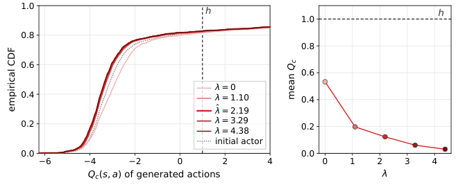
Figure 5 trains the flow actor against the frozen critics of a 1M-step Hopper checkpoint for several fixed multipliers; larger multipliers shift the generated-action cost-critic distribution left, a diagnostic of the implemented update.

Refer to caption — Figure 5: Frozen-critic multiplier response. For each fixed $\lambda$ , a flow actor is trained from the same random initialization (dotted) for the same number of updates. Larger multipliers shift the generated-action cost-critic CDF left. The dashed lines mark the budget $h$ in cost-critic units, and $\hat{\lambda}$ is the multiplier stored in the checkpoint.

Constrained Flow Policy Updates: A Generalized Schrödinger Bridge View

Abstract

1 Introduction

2 Related Work

3 The Constrained Flow-Update Problem

3.1 From an Episodic Constraint to an Actor Objective

3.2 A Direct Actor Update for a Flow Policy

Problem 1 (Direct constrained flow update).

4 A Safety-Tilted Schrödinger Bridge

4.1 From a Reference Process to Kinetic Regularization

Problem 2 (Constrained one-ended Schrödinger bridge).

Problem 3 (Equivalent kinetic-energy reformulation).

4.2 Action-Space Form and Safety Tilt

Theorem 1 (Action-space form).

Theorem 2 (Gibbs solution and safety tilt).

4.3 The Vanishing-Noise Limit

Theorem 3 (Vanishing noise).

5 Practical Online Algorithm

Kinetic-energy adaptation.

6 Experiments

Baselines.

6.1 Main Results

6.2 Ablation Studies

Augmented versus standard Lagrangian.

Effect of the actor family.

7 Conclusion and Limitations

Reproducibility Statement

AI Use Statement

References

Appendix A Extended Related Work

A common frame.

1) Q-value guidance.

2) Weighted matching.

3) Policy gradient.

4) Reparameterization.

Safe RL with Gaussian actors.

Safe RL with generative actors.

Schrödinger-bridge view of policy updates.

Appendix B Proofs and Additional Frozen-Update Results

B.1 Proofs of Theorems 1, 2 and 3

Theorem 4 (Formal version of Theorems 1, 2 and 3).

Path and endpoint divergence.

Endpoint form.

Problems 2 and 3.

Proof.

B.2 The Finite-Step Objective Identity

Corollary 5 (Objective for the midpoint map).

Proof.

B.3 Additional Consequence of the Safety Tilt

B.4 Constructive Positive-Noise Lift of a Terminal Map

B.5 Injectivity of the Vanishing-Noise Map

Appendix C Assumptions and Scope

Appendix D Practical Actor–Critic Implementation

Action squashing.

Solver and kinetic energy.

Budget conversion and multiplier schedule.

Critic targets.

Kinetic-energy coefficient.

Completed-episode feedback.

Appendix E Experimental Details and Additional Results

E.1 Tasks and Evaluation Protocol

E.2 RAFALE Settings

E.3 Baselines

RESPO.

CAL.

RCRL.

ALGD.

E.4 Ablation Protocols

Lagrangian ablation.

Evaluation metrics.

Policy class.

E.5 Additional Results

Seed-level feasibility.

Learning curves against baselines.

Lagrangian-variant curves.

Actor-family curves.

Frozen-critic multiplier response.

Constrained Flow Policy Updates:
A Generalized Schrödinger Bridge View